Grids as Graphs
You already know how to run DFS and BFS on a graph built from adjacency lists. Here's the twist: most competitive-programming graph problems don't give you adjacency lists at all. They give you grids. And the single biggest mistake beginners make is trying to convert that grid into an explicit graph. Don't. The grid itself is the graph.
Every Cell Is a Node
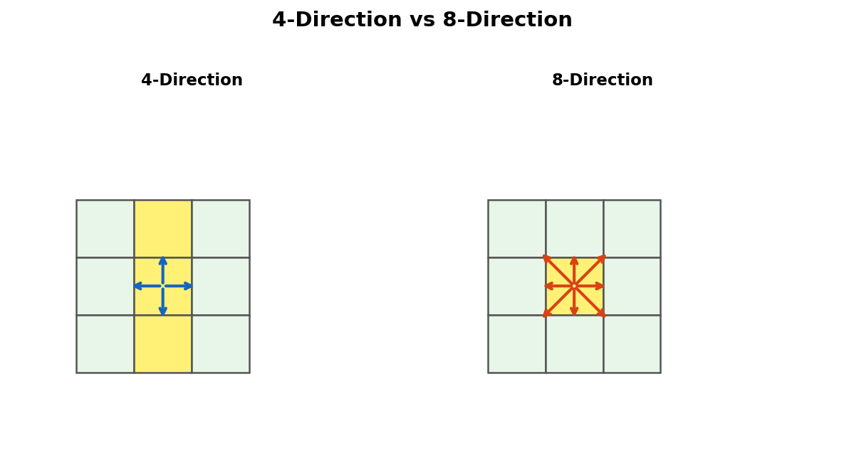
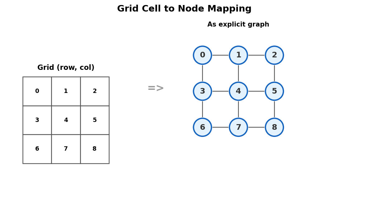
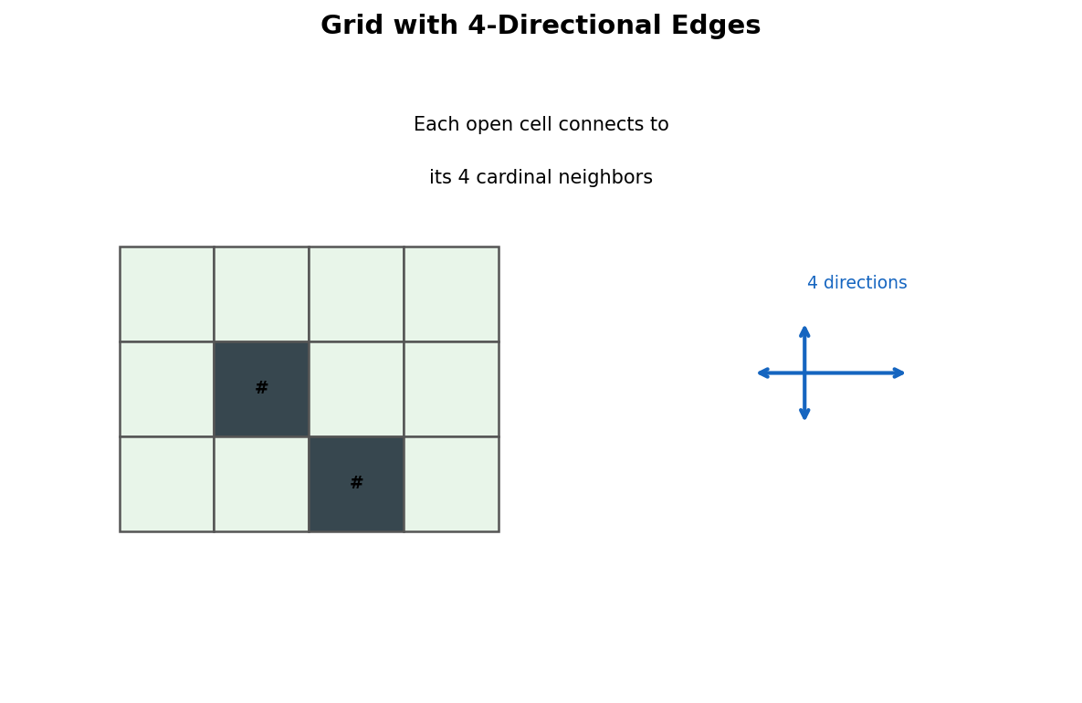
A grid with \(H\) rows and \(W\) columns has \(H \times W\) cells. Each cell \((r, c)\) is a node. Two cells are connected by an edge if they share a side. That's it --- no edge list to read, no adjacency list to build.
This 3x4 grid has 12 nodes. Every . cell connects to its neighbors above, below, left, and right --- provided the neighbor exists and isn't a wall (#). You never enumerate these edges in advance. You compute them on the fly.
Key insight. On an adjacency-list graph, you look up
adj[u]to find neighbors. On a grid, you compute neighbors with arithmetic:(r-1,c),(r+1,c),(r,c-1),(r,c+1). The neighbor function replaces the adjacency list entirely.
The dx/dy Arrays Trick
Manually writing four if statements for up/down/left/right gets ugly fast. Use direction arrays instead.
Now iterate over all four directions in a loop:
for (int d = 0; d < 4; d++) {
    int nr = r + dx[d];
    int nc = c + dy[d];
    // (nr, nc) is a candidate neighbor
}
| Direction | dx | dy | Effect |
|---|---|---|---|
| Right | 0 | +1 | Same row, next column |
| Left | 0 | -1 | Same row, previous column |
| Down | +1 | 0 | Next row, same column |
| Up | -1 | 0 | Previous row, same column |
For 8-directional movement (including diagonals), extend to 8 pairs:
Most grid problems use 4-directional unless stated otherwise.
Gotcha. Some problems define the grid with
(x, y)wherexis the column andyis the row. Read the problem statement carefully. In competitive programming, we almost always use(row, col)where row increases downward.
Bounds Checking
Not every candidate neighbor is valid. A cell on the top edge has no upward neighbor. A cell in a corner has only two neighbors. You must check bounds before accessing the grid.
This check replaces the "does this edge exist?" question you'd ask of an adjacency list. Combine it with a wall check:
if (nr >= 0 && nr < H && nc >= 0 && nc < W
    && grid[nr][nc] == '.' && !visited[nr][nc]) {
    // valid, passable, unvisited neighbor
}
That single if statement is the entire "adjacency list lookup" for grids. Write it once, use it everywhere.
The Visited Array
On adjacency-list graphs, visited is a 1D array indexed by node. On grids, it's a 2D array indexed by (row, col).
Some people skip the visited array entirely and mark cells directly in the grid --- change . to # after visiting. This works when you don't need the original grid afterward.
void dfs(int r, int c) {
    grid[r][c] = '#'; // mark visited by destroying the cell
    for (int d = 0; d < 4; d++) {
        int nr = r + dx[d], nc = c + dy[d];
        if (nr >= 0 && nr < H && nc >= 0 && nc < W
            && grid[nr][nc] == '.') {
            dfs(nr, nc);
        }
    }
}
Gotcha. Modifying the grid in-place saves memory but destroys information. If you need to reference the original grid later (e.g., to check cell types or print the grid), use a separate
visitedarray.
DFS on a Grid
DFS on a grid is identical to DFS on an adjacency list. The only difference is how you find neighbors.
void dfs(int r, int c) {
    visited[r][c] = true;
    for (int d = 0; d < 4; d++) {
        int nr = r + dx[d];
        int nc = c + dy[d];
        if (nr >= 0 && nr < H && nc >= 0 && nc < W
            && !visited[nr][nc] && grid[nr][nc] == '.') {
            dfs(nr, nc);
        }
    }
}
Compare this to the adjacency-list DFS from Chapter 1:
Same structure. The for (int d = 0; d < 4; d++) loop with bounds/wall checking replaces for (int v : adj[u]). That's the entire translation.
Counting Connected Regions
The classic first grid problem: given a grid of . (floor) and # (wall), count how many connected regions of floor exist.
This is identical to counting connected components on an adjacency-list graph. Loop over every cell. If it's floor and unvisited, run DFS from it and increment the counter.
int regions = 0;
for (int i = 0; i < H; i++) {
    for (int j = 0; j < W; j++) {
        if (grid[i][j] == '.' && !visited[i][j]) {
            dfs(i, j);
            regions++;
        }
    }
}
Trace
Grid (4x5):
| Step | Cell | Action | Regions |
|---|---|---|---|
| 1 | (0,0) | Unvisited .. DFS explores (0,0), (0,1), (1,0), (2,0), (2,1), (2,2), (3,2), (3,3), (3,4), (2,4) |
1 |
| 2 | (0,1) | Already visited. Skip. | 1 |
| 3 | (0,3) | Unvisited .. DFS explores (0,3), (0,4), (1,3), (1,4) |
2 |
| ... | ... | Remaining cells all visited or walls. | 2 |
Result: 2 regions.
Key insight. Counting connected regions on a grid is the same algorithm as counting connected components in Chapter 1. The only change is mechanical: how you enumerate neighbors.
BFS on a Grid
BFS works identically. Push the starting cell, pop from the front, expand neighbors.
void bfs(int sr, int sc) {
    queue<pair<int,int>> q;
    q.push({sr, sc});
    visited[sr][sc] = true;
    while (!q.empty()) {
        auto [r, c] = q.front(); q.pop();
        for (int d = 0; d < 4; d++) {
            int nr = r + dx[d], nc = c + dy[d];
            if (nr >= 0 && nr < H && nc >= 0 && nc < W
                && !visited[nr][nc] && grid[nr][nc] == '.') {
                visited[nr][nc] = true;
                q.push({nr, nc});
            }
        }
    }
}
BFS on grids gives you shortest path in number of steps --- every edge has weight 1.
Gotcha. Mark cells visited when you push them, not when you pop them. If you wait until popping, the same cell can be pushed multiple times, wasting time and memory. This is the most common BFS bug on grids.
Complexity
A grid with \(H\) rows and \(W\) columns has \(N = H \times W\) cells and at most \(2N\) edges (each cell has at most 4 neighbors, each edge counted twice). DFS and BFS both run in \(O(H \times W)\) time and space. This matches the \(O(V + E)\) complexity from Chapter 1.
Exercises
-
8-directional regions. Modify the region-counting code to use 8-directional adjacency. On a grid where two
.cells touch only diagonally, should they be in the same region? How does the count change compared to 4-directional? -
Edge counting. Given a grid, count the total number of edges in the implicit graph (only between
.cells). Don't double-count:(r1,c1)-(r2,c2)and(r2,c2)-(r1,c1)is one edge. -
Largest region. Modify DFS to return the size of the region it explores. Find the largest region in the grid. (This is a warmup for Lesson 2.)
-
Border cells. Count how many
.cells lie on the border of the grid (row 0, row H-1, col 0, col W-1). For each such cell, determine which connected region it belongs to. How many distinct regions touch the border?
Problems
| Problem | Link | Difficulty |
|---|---|---|
| CSES Counting Rooms | cses.fi/problemset/task/1192 | Easy |
| LC 200 --- Number of Islands | leetcode.com/problems/number-of-islands | Medium |
| LC 733 --- Flood Fill | leetcode.com/problems/flood-fill | Easy |
| LC 1020 --- Number of Enclaves | leetcode.com/problems/number-of-enclaves | Medium |