1D DP Optimization
The Pattern
Here's a DP recurrence you'll see over and over:
In words: to compute dp[i], you look back at the last K states, pick the best one, and add some cost.
Brute force computes this in O(K) per state, giving O(NK) total. When N and K are both up to 10^5 or 10^6, that's too slow.
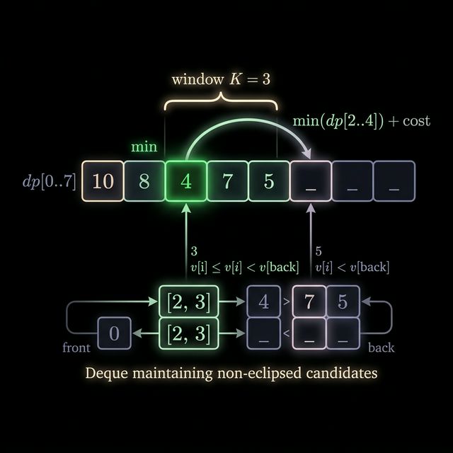
But look at what's happening as i increases by 1. The range [i - K, i - 1] slides forward by one position. The left boundary moves right (an old state drops out), and the right boundary moves right (a new state enters).
That's a sliding window. And finding the minimum over a sliding window is exactly what the monotonic queue does.
The Jump Game
Let's make this concrete with a problem.
Problem: You're at position 0 of an array of N integers. From position i, you can jump to any position from i+1 to i+K. Landing on position j costs cost[j]. Find the minimum total cost to reach position N-1.
Recurrence:
Each dp[i] is the cheapest way to reach position i. To get there, you jumped from some position j that's at most K steps behind, and the cost of that path was dp[j]. Then you pay cost[i] for landing.
With brute force, for each i you'd scan backwards up to K positions. That's O(NK).
Applying the Monotonic Queue
The key observation: as i moves from 1 to N-1, the window of valid predecessors [i-K, i-1] slides forward. We need min(dp[j]) over this window.
This is the sliding window minimum problem from lesson 1 — except the values we're tracking are dp[j] instead of a[j], and we're building the dp array as we go.
Here's the plan:
- Maintain a deque of indices, ordered so that
dp[dq.front()]is the smallest in the window. - For each i, expire any front index that's too far back.
- Use
dp[dq.front()]as the best predecessor to computedp[i]. - Eclipse from the back — any index with a worse dp value than
dp[i]will never be chosen. - Push i onto the deque.
vector<long long> dp(n, LLONG_MAX);
dp[0] = cost[0];

deque<int> dq;
dq.push_back(0);

for (int i = 1; i < n; i++) {
    // Expire
    if (!dq.empty() && dq.front() < i - k)
        dq.pop_front();

    // Transition
    if (!dq.empty())
        dp[i] = dp[dq.front()] + cost[i];

    // Eclipse
    while (!dq.empty() && dp[dq.back()] >= dp[i])
        dq.pop_back();

    dq.push_back(i);
}

cout << dp[n - 1] << "\n";
Total time: O(N). Each index enters and leaves the deque at most once.
Walking Through It
Array: cost = [10, 15, 20, 9, 2, 7], K = 3
i = 0: Base case. dp[0] = 10. Deque: [0].
i = 1: Expire: front is 0, range is [0, 0]. In range. Transition: dp[1] = dp[0] + 15 = 25. Eclipse: dp[0] = 10 < 25, no pop. Push 1. Deque: [0, 1].
i = 2: Expire: front 0, range [0, 1]. In range. Transition: dp[2] = dp[0] + 20 = 30. Eclipse: dp[1] = 25 < 30. Push 2. Deque: [0, 1, 2].
i = 3: Expire: front 0, range [0, 2]. In range. Transition: dp[3] = dp[0] + 9 = 19. Eclipse: dp[2] = 30 >= 19, pop. dp[1] = 25 >= 19, pop. dp[0] = 10 < 19, stop. Push 3. Deque: [0, 3].
i = 4: Expire: front 0, range [1, 3]. Index 0 is out! Pop front. Deque: [3]. Transition: dp[4] = dp[3] + 2 = 21. Eclipse: dp[3] = 19 < 21, no pop. Push 4. Deque: [3, 4].
i = 5: Expire: front 3, range [2, 4]. In range. Transition: dp[5] = dp[3] + 7 = 26. Eclipse: dp[4] = 21 < 26, no pop. Push 5. Deque: [3, 4, 5].
Answer: dp[5] = 26.
The optimal path is: 0 -> 3 -> 5, with costs 10 + 9 + 7 = 26.
Notice at i = 4 how the old champion (index 0 with dp = 10) expired. Without the deque, we might have wasted time scanning dead indices. With it, one front pop and we're done.
Recognizing the Pattern
Not every DP problem can be optimized this way. Here's what to look for:
It works when:
- The recurrence is
dp[i] = min/max(dp[j]) + f(i)for j in some sliding range. - The range of valid j values slides forward as i increases.
- The function
f(i)depends only on i, not on j. (This is the important part.)
It doesn't work when:
- The cost depends on both i and j in a non-separable way:
dp[i] = min(dp[j] + g(i, j))whereg(i, j)can't be split intof(i) + h(j). - The range of valid j values doesn't move monotonically.
When the cost can be separated — meaning you can rewrite dp[j] + g(i, j) as (dp[j] + h(j)) + f(i) — then you're querying min(dp[j] + h(j)) over a sliding window, and the monotonic queue still applies. You just store dp[j] + h(j) as the value associated with index j.
What Comes Next
This lesson covers the "simple" case: the thing we're minimizing over the window is just dp[j] (or dp[j] + h(j) for some function of j alone). The f(i) part factors out cleanly.
But what if the cost is dp[j] + slope * (i - j) for some varying slope? What if the relationship between i and j is linear, and the optimal j depends on the "slope" at position i?
That's the Convex Hull Trick, which shows up in Chapter 6. It handles the case where the transition cost is a linear function of j, and different values of i "prefer" different slopes. The monotonic queue can't handle that — you need a different geometric structure.
For now, the rule of thumb: if you can separate the i-part from the j-part, and the valid range of j slides forward, reach for the monotonic queue.
One More Thing: The Expiration Condition
A subtle point that's easy to get wrong. In the sliding window min/max problem, the expiration check was:
In the DP problem, it's:
Why the difference? In the window problem, the window for position i is [i - k + 1, i], so an index j is expired when j <= i - k, which is the same as j < i - k + 1.
In the DP problem, the valid predecessors are [i - k, i - 1] — you can jump up to K steps. So an index j is expired when j < i - k.
The point: always think carefully about the exact bounds of your window. Off-by-one errors here will give you wrong answers that are maddeningly close to correct.
Try It
The starter code implements the jump game problem. The expire and eclipse steps are left blank. Fill them in using the pattern from this lesson.
Input format: Line 1: N K Line 2: N integers (the cost array)
Output: the minimum cost to reach position N-1.
Test with the example above: 6 3 and 10 15 20 9 2 7. The answer should be 26.