B-Trees, LSM Trees & Hash Indexes

TL;DR

B-trees give you fast reads by keeping data sorted in a balanced tree structure. LSM trees give you fast writes by buffering in memory and flushing sequentially. Hash indexes give you O(1) equality lookups but can't do range queries. Every database picks a side in the read-vs-write trade-off.

The Library Card Catalog

Imagine a library with 10 million books. You need to find one specific title. Without any organization, you'd walk every aisle, scanning every shelf. That's a full table scan.

Now imagine the library has a card catalog — a set of drawers organized alphabetically. You open the "M" drawer, flip to "Mo," find "Moby Dick," and the card tells you "Aisle 14, Shelf 3, Position 7." Three lookups instead of scanning millions of spines.

That card catalog is an index. And the way those cards are organized — sorted, layered, balanced — is the B-tree.

B-Trees — The Default Index Everywhere

The B-tree (short for "balanced tree," though the inventor never confirmed this) is the most widely used index structure in databases. PostgreSQL uses B-trees by default. MySQL InnoDB uses a variant called B+ trees. SQLite, Oracle, SQL Server — all B-trees under the hood.

The Structure

A B-tree is a self-balancing tree where every node is a page — a fixed-size block of data, typically 8 KB in PostgreSQL. Each page holds sorted keys and pointers to child pages.

                    [35 | 70]                         ← Root page (Level 0)
                   /    |    \
          [10|20|30] [45|55|60] [80|90|95]            ← Internal pages (Level 1)
          / | | \    / | | \    / | | \
        [leaves]   [leaves]   [leaves]                ← Leaf pages (Level 2)

• Root node: The single entry point. Always in memory (buffer pool).
• Internal nodes: Contain keys and pointers that guide the search left or right.
• Leaf nodes: Contain the actual indexed values and pointers to the heap page where the full row lives.

Why 3-4 Levels Covers Millions of Rows

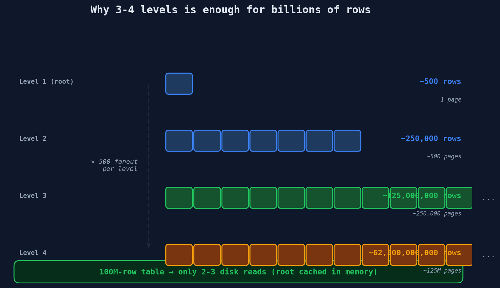
Here's the math that makes B-trees magical. Each page is 8 KB. A typical B-tree node can hold around 500 keys (depending on key size). So:

Tree Depth	Max Rows Indexed
1 level (root only)	~500
2 levels	~250,000
3 levels	~125,000,000
4 levels	~62,500,000,000

Three levels covers 125 million rows. Four levels covers 62 billion. Since the root page is always cached in memory, a lookup in a table with 100 million rows requires just 2-3 disk reads. That's why B-tree lookups are effectively O(log N) but with a very large branching factor that keeps the constant tiny.

How a B-Tree Lookup Works — Step by Step

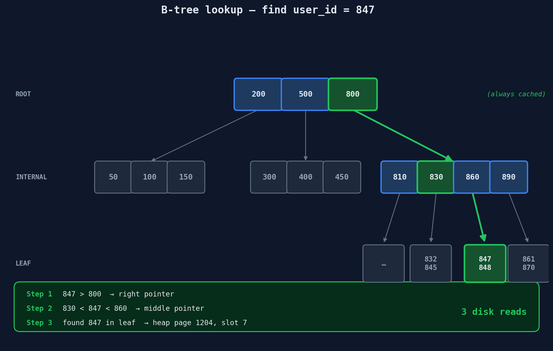
Let's trace finding user_id = 847 in a B-tree index:

Step 1: Read root page (cached in memory)
        [200 | 500 | 800]
        847 > 800 → go right

Step 2: Read internal page (1 disk read)
        [810 | 830 | 860 | 890]
        847 > 830 and 847 < 860 → go to child between 830 and 860

Step 3: Read leaf page (1 disk read)
        [..., 845, 846, 847, 848, ...]
        Found! 847 → heap page 1204, slot 7

Step 4: Read heap page 1204 (1 disk read)
        Return the full row

Total: 3 disk reads. Compare that to scanning 10,000+ pages sequentially. This is why every database uses B-trees as the default.

In-Place Updates and Write Behavior

When you insert a new key, the B-tree finds the correct leaf page and adds the key in sorted order. If the page is full, it splits into two pages and pushes the middle key up to the parent. This splitting is what keeps the tree balanced — no branch ever gets much deeper than another.

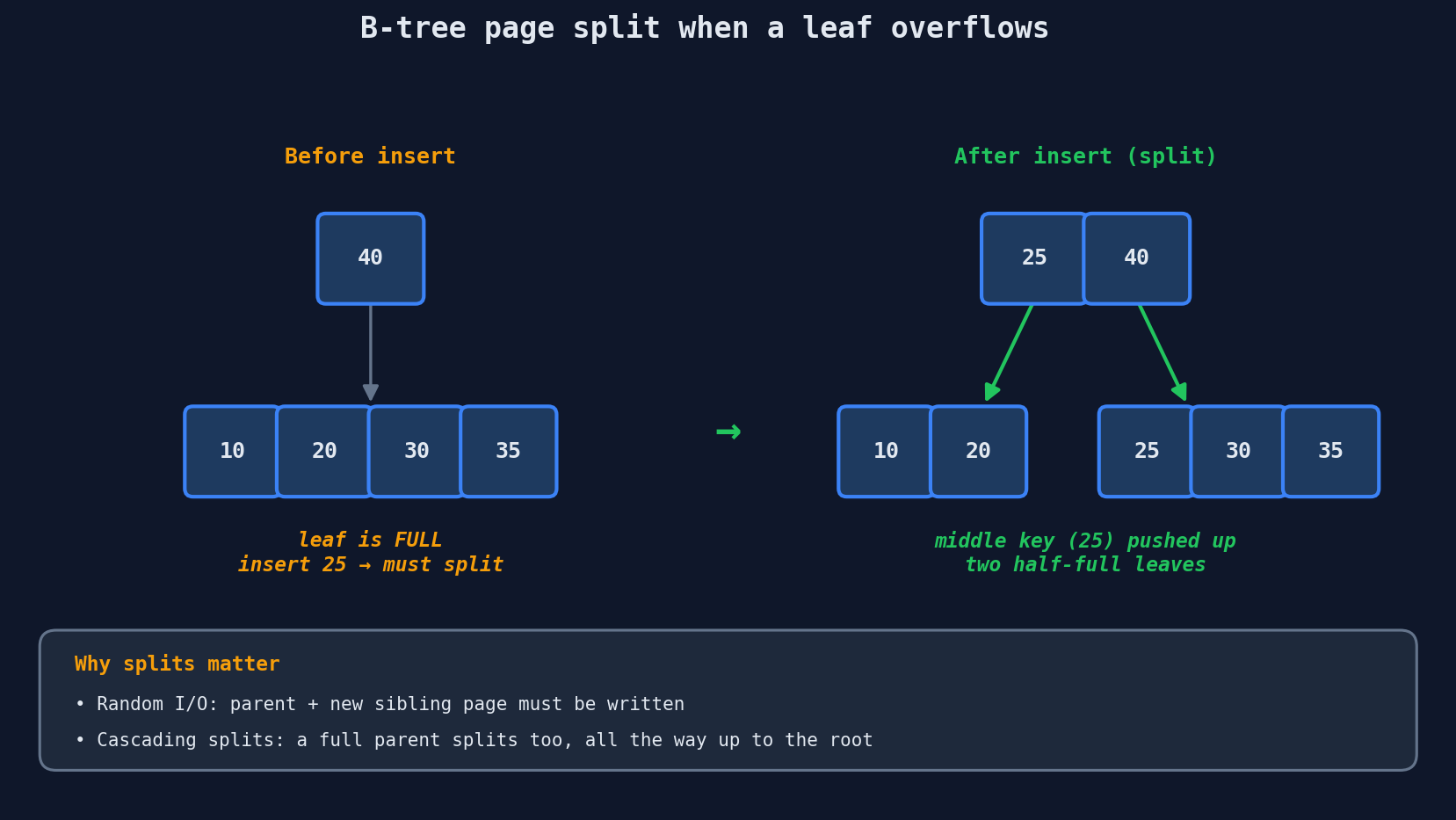
Updates modify the leaf page in place. Deletes mark the key as removed (and the space gets reclaimed later). All of this involves random I/O — jumping to specific pages on disk. That's fine for reads, but it becomes a bottleneck for write-heavy workloads.

Interview Tip

When an interviewer asks "what index type would you use?" — the answer is almost always a B-tree unless you have a specific reason not to. It's the default for a reason: excellent read performance, decent write performance, and support for both equality and range queries.

LSM Trees — Optimized for Writes

What if your workload is 90% writes? Think of a time-series database ingesting millions of sensor readings per second, or a messaging system like Discord storing billions of messages. Random in-place updates on a B-tree become a bottleneck.

The Log-Structured Merge Tree (LSM tree) takes a fundamentally different approach: instead of updating data in place, it buffers writes in memory and flushes them to disk as sorted, immutable files.

How LSM Trees Work

1. WRITE arrives
      ↓
2. Insert into MEMTABLE (in-memory sorted structure, typically a red-black tree)
      ↓ (when memtable is full, ~64MB)
3. Flush to disk as an SSTABLE (Sorted String Table) — one sequential write
      ↓ (over time, SSTables accumulate)
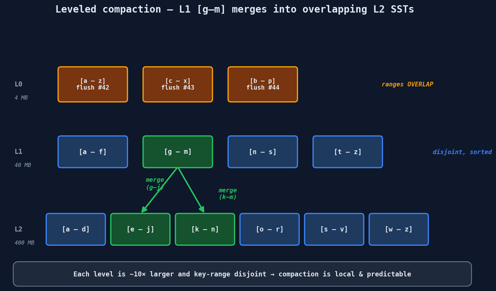
4. COMPACTION merges multiple SSTables into larger, sorted ones

Here's the core mechanism stripped to its essence:

from sortedcontainers import SortedDict

class TinyLSM:
    def __init__(self, flush_threshold=1000):
        self.memtable = SortedDict()         # in-memory sorted structure
        self.sstables = []                    # flushed files on disk (newest first)
        self.flush_threshold = flush_threshold

    def put(self, key, value):
        self.memtable[key] = value           # write to memory — no disk I/O
        if len(self.memtable) >= self.flush_threshold:
            self.sstables.insert(0, dict(self.memtable))  # flush as immutable file
            self.memtable.clear()

    def get(self, key):
        if key in self.memtable:             # check memory first
            return self.memtable[key]
        for table in self.sstables:          # then check each SSTable, newest first
            if key in table:
                return table[key]
        return None                          # not found

Writes never touch disk until the flush. That's why LSM trees handle millions of writes per second.

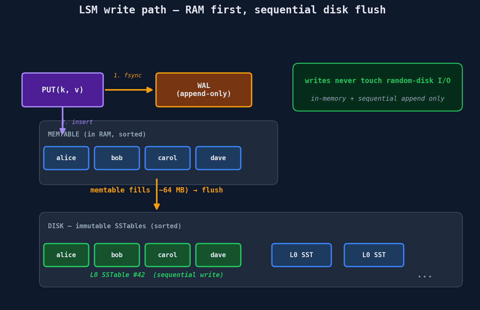
Memtable: An in-memory sorted data structure (red-black tree or skip list). All writes go here first. This is blazing fast — no disk I/O at all.

SSTable (Sorted String Table): When the memtable fills up, it gets written to disk as a single sorted file. This is a sequential write — the fastest thing you can do on disk. No random seeks.

Compaction: Over time, you accumulate many SSTables. Background threads merge them together, removing deleted keys and combining updates. This keeps read performance from degrading.

The Read Path (Where LSM Trees Pay)

Reading from an LSM tree is more complex:

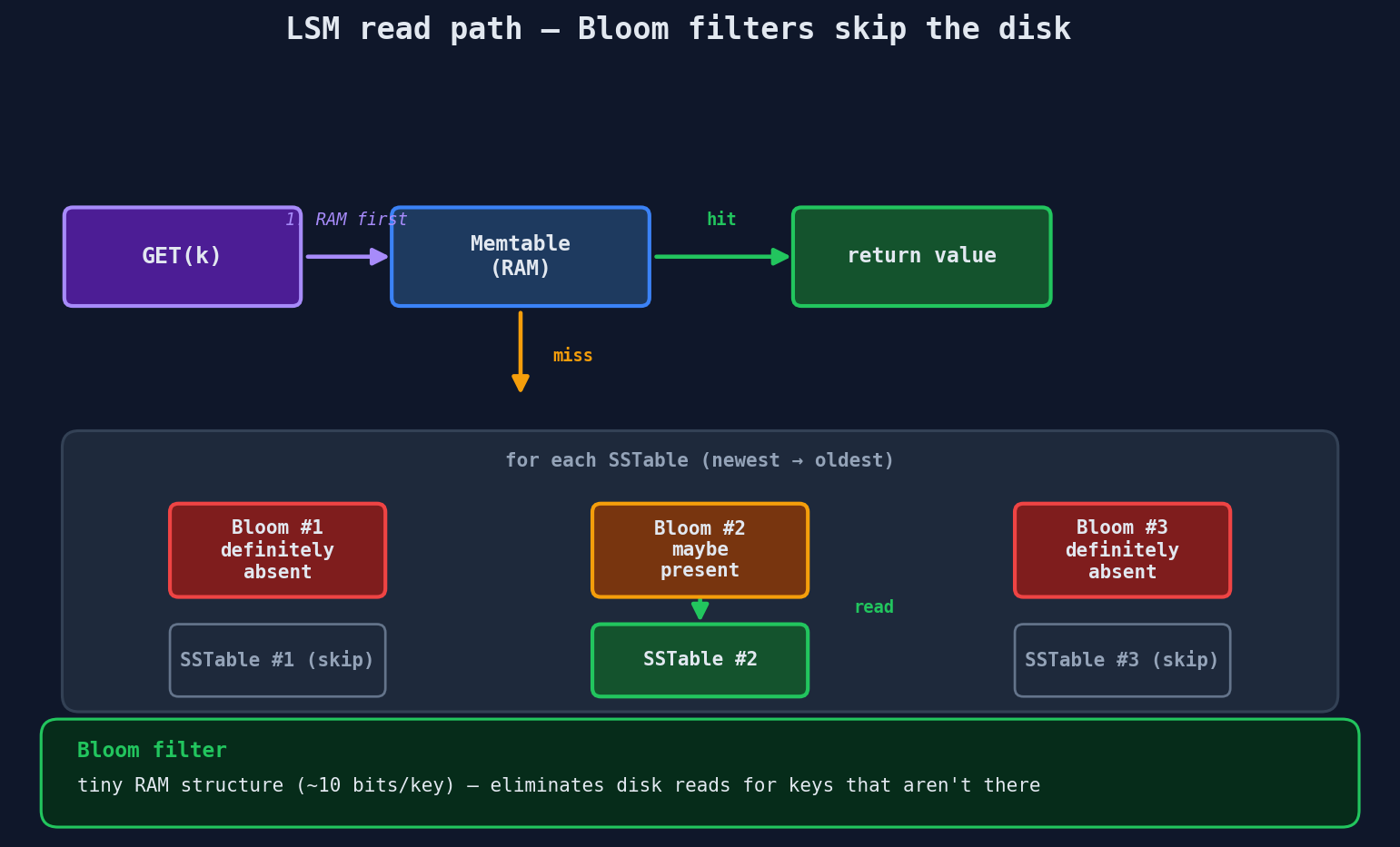
1. Check the memtable (in memory — fast)
2. Check the most recent SSTable on disk
3. Check the next SSTable
4. ... keep checking older SSTables until found

This is called read amplification — a single read might check multiple files. To mitigate this, LSM trees use Bloom filters at each level: a probabilistic data structure that can tell you "this key is definitely NOT in this SSTable" without reading the file. This skips most unnecessary checks.

Who Uses LSM Trees?

• Cassandra — LSM trees for its storage engine
• RocksDB (by Facebook) — embedded LSM tree used inside dozens of systems
• LevelDB (by Google) — the predecessor to RocksDB
• DynamoDB — uses an LSM-style engine internally
• ScyllaDB — Cassandra-compatible with LSM storage

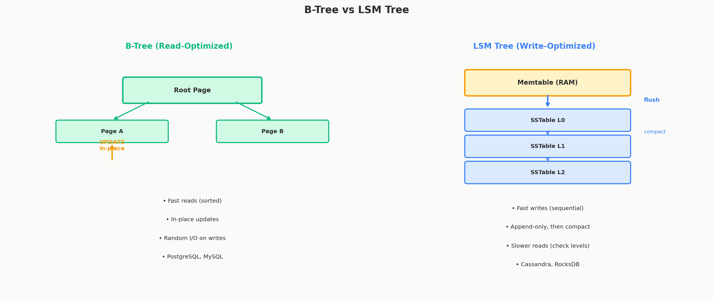
The Big Trade-Off: B-Trees vs LSM Trees

This is one of the most important trade-offs in database engineering. There are three types of "amplification" — and you can only optimize for two out of three:

Amplification Type	What It Means	B-Tree	LSM Tree
Read amplification	How many disk reads per query	Low (3-4 reads)	Higher (check multiple SSTables)
Write amplification	How many times data is written to disk	Higher (in-place updates, page splits)	Lower (sequential writes, but compaction re-writes)
Space amplification	How much extra disk space is used	Low (one copy of data)	Higher (multiple SSTables may have same key during compaction)

The rule of thumb:

• B-trees optimize for reads — in-place updates mean data is always where you expect it
• LSM trees optimize for writes — sequential I/O is 10-100x faster than random I/O

Feature	B-Tree	LSM Tree
Read latency	Predictable, fast	Variable (may check multiple levels)
Write throughput	Good	Excellent (sequential writes)
Space usage	Efficient	Can temporarily use 2x space during compaction
Range queries	Excellent	Good (within each SSTable)
Concurrency	Page-level locking	Append-only, minimal lock contention
Used by	PostgreSQL, MySQL, Oracle	Cassandra, RocksDB, LevelDB, DynamoDB
Best for	OLTP with mixed reads/writes	Write-heavy, time-series, logging

Interview Tip

If an interviewer describes a write-heavy workload (logging, event streaming, IoT telemetry), mention that an LSM-tree-based database like Cassandra or RocksDB would handle the write throughput better than a B-tree-based system. Then explain ~~why~~ — sequential writes vs random I/O. That shows deep understanding.

Hash Indexes — O(1) But Limited

A hash index is the simplest index type. It hashes the key and maps it directly to a location. Think of it like a Python dictionary — you give it a key, it gives you the value in constant time.

hash("alice@example.com") → bucket 4,271 → heap page 847, slot 3

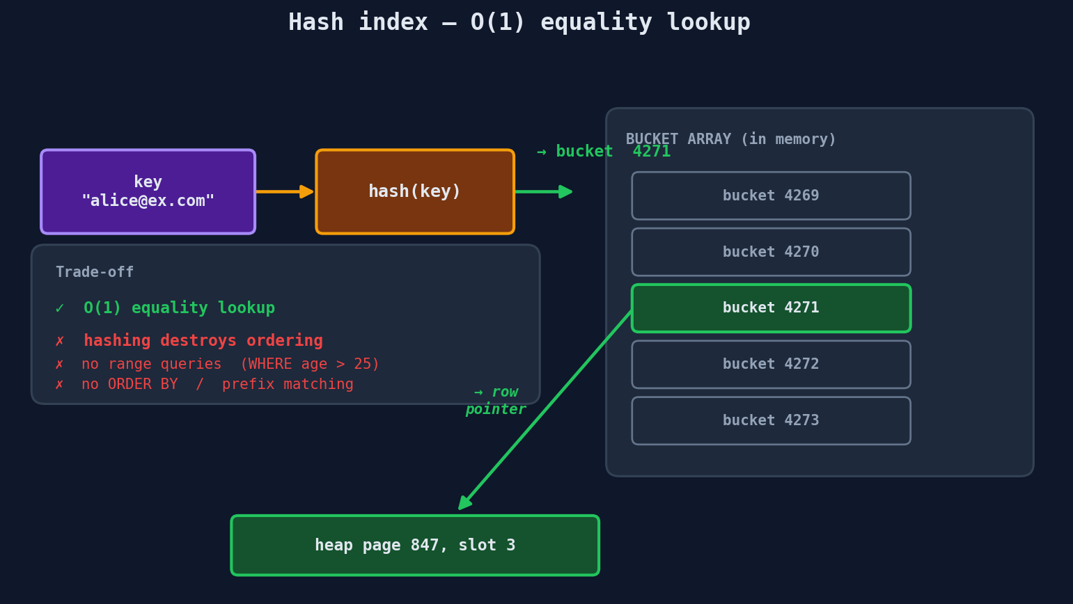
Strengths: - O(1) equality lookups — the fastest possible for exact-match queries - Simple implementation

Weaknesses: - No range queries — WHERE age > 25 can't use a hash index because hashing destroys ordering - No sorting — ORDER BY can't leverage a hash index - No partial matching — WHERE name LIKE 'Al%' needs ordered data

PostgreSQL supports hash indexes (they became crash-safe in version 10), but they're rarely used directly. Where hash indexes shine is ~~internally~~ — databases use hash tables for hash joins (joining two tables by hashing the join key) and for in-memory lookup structures.

The Full Comparison

Feature	B-Tree	LSM Tree	Hash Index
Lookup	O(log N)	O(log N) across levels	O(1)
Range queries	Yes	Yes	No
Write speed	Moderate	Fast (sequential)	Fast
Read speed	Fast	Moderate	Fastest (equality)
Space overhead	Moderate	Higher (compaction)	Low
Ordering	Maintained	Within SSTables	None
Default in	PostgreSQL, MySQL	Cassandra, RocksDB	Internal use (hash joins)

Quick Recap

Concept	Key Insight	When to Use
B-tree	Sorted, balanced, 3-4 levels covers millions of rows	General purpose — reads, writes, range queries
LSM tree	Buffer in memory, flush sequentially, compact in background	Write-heavy workloads — logging, time-series, messaging
Hash index	O(1) equality but no range queries	Exact-match lookups only, internal hash joins
Read amplification	Number of disk reads per query	B-trees win
Write amplification	Number of times data is written to disk	LSM trees win
Space amplification	Extra disk space consumed	B-trees win