Streaming Data
Every chapter so far assumed you had the full array upfront. But what if data arrives one element at a time, forever? Welcome to streaming.
The Problem
Imagine a temperature sensor that sends a reading every second. You need the minimum temperature in the last 60 seconds at all times. Not the minimum of all time — the minimum of the most recent 60 values.
The naive approach: store a circular buffer of the last 60 readings, scan it for the minimum each time. That's O(K) per reading, where K is the window size. For K = 60, maybe that's fine. For K = 100,000 (say, a rolling minimum over the last 100K stock ticks), it's not.
And here's the real constraint: the stream never stops. You can't store the entire history and post-process it. You need to answer "what's the minimum right now?" as each new value arrives. O(1) amortized per element. Sound familiar?
The Monotonic Deque, Revisited
You already built this in Chapter 2. The sliding window min/max deque handles exactly this scenario. The only difference is that in Chapter 2, you had an array of N elements and iterated through it. In a streaming context, N is infinite — values arrive one at a time, and you process each one immediately.
The mechanics are identical:
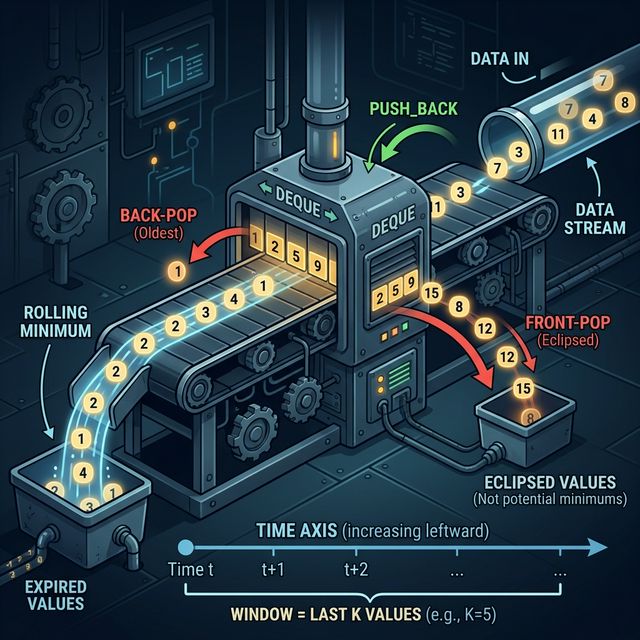
- Expire — remove the front element if its timestamp is too old (more than K steps ago).
- Eclipse — remove elements from the back that the new value dominates.
- Push — add the new value (with its timestamp) to the back.
- Read — the front of the deque is the current answer.
The key shift is that instead of storing array indices, we store timestamps. Each incoming value gets a monotonically increasing timestamp. The expiration check becomes: "is the front element's timestamp older than current_time - K?"
Walking Through a Stream
Let's trace this with a concrete scenario. A temperature sensor sends readings, and we want the rolling minimum over the last 5 readings (K = 5).
Stream arrives: 72, 68, 71, 65, 73, 70, 69, 74, ...
t=0, val=72: Deque empty. Push {72, 0}. Deque: [{72,0}]. Min: 72.
t=1, val=68: Eclipse: 72 >= 68, pop it. Deque empty. Push {68, 1}. Deque: [{68,1}]. Min: 68.
t=2, val=71: Eclipse: 68 < 71, stop. Push {71, 2}. Deque: [{68,1}, {71,2}]. Min: 68.
t=3, val=65: Eclipse: 71 >= 65, pop. 68 >= 65, pop. Push {65, 3}. Deque: [{65,3}]. Min: 65.
t=4, val=73: Eclipse: 65 < 73, stop. Push {73, 4}. Deque: [{65,3}, {73,4}]. Min: 65.
t=5, val=70: Expire: front is {65, 3}, window is [1, 5]. Timestamp 3 >= 1, so it's still in range. Eclipse: 73 >= 70, pop. 65 < 70, stop. Push {70, 5}. Deque: [{65,3}, {70,5}]. Min: 65.
t=6, val=69: Expire: front is {65, 3}, window is [2, 6]. Timestamp 3 >= 2, still valid. Eclipse: 70 >= 69, pop. 65 < 69, stop. Push {69, 6}. Deque: [{65,3}, {69,6}]. Min: 65.
t=7, val=74: Expire: front is {65, 3}, window is [3, 7]. Timestamp 3 >= 3, still valid (barely). Eclipse: 69 < 74, stop. Push {74, 7}. Deque: [{65,3}, {69,6}, {74,7}]. Min: 65.
t=8, val=??: Whatever arrives, the first thing that happens is expiration. The window becomes [4, 8]. Front timestamp is 3, which is less than 4. Pop it. Now 65 is gone. The deque becomes [{69,6}, {74,7}]. The new minimum jumps up to 69 — unless the incoming value is smaller.
Notice: by t=8, we've processed 9 readings but the deque never held more than 3 elements. Millions of readings could flow through, and the deque stays tiny. That's the power of lossy compression.
Lossy Compression — The Deep Insight
Think about what the monotonic deque is actually doing. It's compressing the stream. Not losslessly — it throws away most values. But it throws away exactly the values that don't matter.
If a value arrives and it's larger than the current minimum, the deque keeps it around just in case — maybe it'll become the minimum after the current minimum expires. But if a value arrives and it's smaller than everything in the deque, it wipes them all out. Those old values can never be the answer again. They've been eclipsed.
This is the same eclipse logic from Chapter 1, now applied to a potentially infinite stream. The deque doesn't remember the stream's history. It remembers a compressed summary: the "candidates" that could still be the answer for some future window position. Everything else is gone.
The space is O(K) in the worst case (if you get a perfectly sorted increasing sequence, every element in the window is a candidate). But in practice, with noisy real-world data, the deque is much smaller. Random data keeps the deque at around O(log K) elements on average.
Where This Shows Up in the Real World
Rate Limiters
Your API server needs to enforce "no more than 1000 requests per minute." You need to track the count of requests in a sliding 60-second window. A monotonic deque variant tracks the running sum efficiently. More precisely, you maintain timestamps of requests and use a sliding window count — but the same deque-style expiration logic applies.
Some rate limiters go further: they track the maximum request rate in any 10-second sub-window within the last minute. That's directly a sliding window maximum — exactly what our deque does.
Anomaly Detection
You're monitoring server response times. Normal latency is 50-200ms. You maintain the rolling minimum and maximum over the last 1000 requests. If a new reading is more than 3x the rolling minimum, or more than 2x the rolling maximum, you flag it as anomalous.
The deque gives you the rolling min and max in O(1) per request. No need to scan the last 1000 values. Two deques — one for min, one for max — and you have a lightweight anomaly detector.
Time-Series Databases
Tools like Prometheus, InfluxDB, and TimescaleDB support queries like "give me the 5-minute moving minimum of CPU usage." Under the hood, these systems use sliding window aggregation algorithms. The monotonic deque is one of the core building blocks.
When you write a PromQL query like min_over_time(cpu_usage[5m]), the engine is doing essentially what you coded in Chapter 2 — maintaining a structure that efficiently tracks the minimum over a sliding time window.
Stock Trading Systems
Trading platforms compute rolling statistics constantly. Stop-loss triggers need the rolling minimum price. Bollinger bands use rolling averages and standard deviations. High-frequency trading systems compute rolling min/max over tick windows to detect breakouts.
The latency requirements are extreme — microseconds per update. A naive O(K) scan per tick is unacceptable. The O(1) amortized deque is standard practice.
The Implementation Difference: Arrays vs. Streams
In Chapter 2, we stored indices into a known array:
In a stream, there's no persistent array. Values arrive and may be discarded. So we store the value alongside its timestamp:
We could also use a circular buffer and store indices into it. But storing pairs is simpler and avoids index-wrapping arithmetic.
The expiration check changes from dq.front() <= i - k to dq.front().second <= t - k. The eclipse check changes from a[dq.back()] >= a[i] to dq.back().first >= val. Same logic, different bookkeeping.
Try It
The starter code reads K, then reads integers one at a time (terminated by -1). After each input, it should print the current minimum of the last K values. If fewer than K values have arrived so far, print the minimum of everything seen.
Fill in the expire and eclipse steps. The logic is the same four-step pattern from Chapter 2, adapted for streaming with timestamps.
Once it works, think about this: how would you extend it to track both the rolling min and the rolling max simultaneously? You'd maintain two deques in parallel — one increasing (for min) and one decreasing (for max). Each incoming value goes through both deques. That gives you a rolling range (max - min) for free, which is the basis of many anomaly detection systems.
What to Take Away
The monotonic deque isn't just an algorithm for competitive programming. It's a streaming primitive — a small, efficient data structure that compresses a potentially infinite stream into just the information you need. Rate limiters, anomaly detectors, time-series databases, and trading systems all use this idea, whether they call it a "monotonic deque" or not.
The core principle hasn't changed since Chapter 1: discard what can't possibly be the answer. In Chapter 1, you discarded elements that were eclipsed by a neighbor. In Chapter 2, you also discarded elements that expired out of a window. Here, the window slides over an infinite stream instead of a finite array. The algorithm is the same. The scale is different.