Decoupled Sweeps

Here's Something That Takes a While to Click

Some greedy problems look like they have one cost function. You stare at them, try a greedy rule, and it almost works — but there is a tension you cannot resolve. Improving one thing worsens another. You try to juggle both at once and get buried in casework.

Here is the reframe. Instead of asking "how do I optimize these two things simultaneously?", ask: "what if I optimized them separately, then stitched the answers together?"

That is a decoupled sweep. Two independent passes, one merge. This lesson is about recognizing when that decomposition is possible and executing it cleanly.

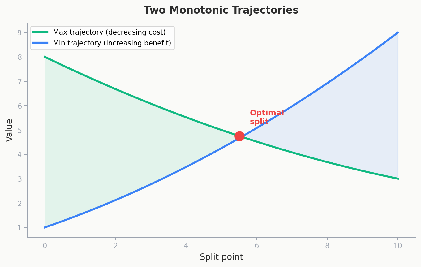
Look at the diagram above. The intuition is physical: one curve (prefix-best) improves as you move right, the other (suffix-best) improves as you move left. They cross at the optimal split point. You never need to search a 2D space — you just sweep along the x-axis.

---

The Core Idea

Problem shape. You need to maximize (or minimize) something that decomposes as:

\[\text{answer} = \max_{i} \left[ f(\text{left half up to } i) + g(\text{right half from } i+1) \right]\]

where \(f\) depends only on elements \(0..i\) and \(g\) depends only on elements \(i+1..n-1\).

The three-step recipe:

1. Prefix array for \(f\). Scan left to right. At each index \(i\), record the best \(f\)-value achievable using elements \(0..i\). This sweep is self-contained — it does not know about \(g\).

2. Suffix array for \(g\). Scan right to left. At each index \(i\), record the best \(g\)-value achievable using elements \(i..n-1\). This sweep is also self-contained.

3. Sweep the split point. For each boundary \(i\), combine bestLeft[i] and bestRight[i+1]. Take the best combination.

Each sweep is \(O(N)\). Total: \(O(N)\). Compare that to \(O(N^2)\) if you tried every pair.

---

Warm-Up: Best Time to Buy and Sell Stock

Problem (LeetCode 121). Given daily prices \(p[0..n-1]\), find the maximum profit from one buy-then-sell. You must buy before you sell.

The Greedy Choice: Don't optimize buy and sell simultaneously. Build the best buy price as a prefix array, the best sell price as a suffix array, and sweep the split point.

The Trap

The brute-force approach: try every pair (buy_day, sell_day) with buy_day \(<\) sell_day. That is \(O(N^2)\). You might try "find the global min and global max" — but the global min might come after the global max. You cannot fix buy and sell independently because they have an ordering constraint.

Here is where almost every first implementation breaks: people try a single pass tracking just the running minimum, computing stockPrices[i] - runningMin at each step. That actually works for this problem, but it does not generalize. The three-pass structure we are about to build extends to harder variants (two transactions, \(k\) transactions) where the single-pass trick falls apart.

Why It Fits the Pattern

Profit \(= p[\text{sell\_day}] - p[\text{buy\_day}]\) where buy_day \(<\) sell_day. This is a spread between two positions. The buy depends on the left portion, the sell depends on the right portion.

• \(f(0..i) =\) minimum price in \(0..i\) (best buy)
• \(g(i+1..n-1) =\) maximum price in \(i+1..n-1\) (best sell)
• answer \(= \max\) over split points of \(g(i+1) - f(i)\)

Full State Trace

Stare at this table. Each row shows the state of both timelines at each index.

Prices: [7, 1, 5, 3, 6, 4]

Pass 1 — Prefix Min (left to right):

Day \(i\)	Price	minPriceSoFar[\(i\)]	Reasoning
0	7	7	Only option
1	1	1	\(\min(7, 1) = 1\)
2	5	1	\(\min(1, 5) = 1\)
3	3	1	\(\min(1, 3) = 1\)
4	6	1	\(\min(1, 6) = 1\)
5	4	1	\(\min(1, 4) = 1\)

Pass 2 — Suffix Max (right to left):

Day \(i\)	Price	maxPriceFuture[\(i\)]	Reasoning
5	4	4	Only option
4	6	6	\(\max(6, 4) = 6\)
3	3	6	\(\max(3, 6) = 6\)
2	5	6	\(\max(5, 6) = 6\)
1	1	6	\(\max(1, 6) = 6\)
0	7	7	\(\max(7, 6) = 7\)

Pass 3 — Sweep split point (both timelines merged):

Split \(i\)	minPriceSoFar[\(i\)]	maxPriceFuture[\(i+1\)]	Profit
0	7	6	-1
1	1	6	5
2	1	6	5
3	1	6	5
4	1	4	3

Answer: 5 (buy at 1 on day 1, sell at 6 on day 4).

Code

int maxProfit(vector<int>& stockPrices) {
    int numDays = stockPrices.size();
    if (numDays < 2) return 0;

    vector<int> minPriceSoFar(numDays);
    minPriceSoFar[0] = stockPrices[0];
    for (int i = 1; i < numDays; i++)
        minPriceSoFar[i] = min(minPriceSoFar[i - 1], stockPrices[i]);

    vector<int> maxPriceFuture(numDays);
    maxPriceFuture[numDays - 1] = stockPrices[numDays - 1];
    for (int i = numDays - 2; i >= 0; i--)
        maxPriceFuture[i] = max(maxPriceFuture[i + 1], stockPrices[i]);

    int maxSingleProfit = 0;
    for (int i = 0; i < numDays - 1; i++)
        maxSingleProfit = max(maxSingleProfit, maxPriceFuture[i + 1] - minPriceSoFar[i]);

    return maxSingleProfit;
}

You can condense this to one pass with a running min, but the three-pass structure generalizes. The next problem demands it.

Try It

Before reading the code, answer this: what happens if prices are strictly decreasing, like [9, 7, 4, 2, 1]? What does each sweep produce, and what is the final answer? Work through the three passes by hand.

---

Leveling Up: Buy and Sell Stock III (Two Transactions)

Problem (LeetCode 123). Same setup as above, but now you can make at most two buy-sell transactions. The transactions cannot overlap (you must sell before buying again). Maximize total profit.

The Trap

With one transaction, you could use a running minimum. With two, you need to find the best pair of non-overlapping transactions. The brute-force approach: try every split point \(i\), compute the best single transaction in \([0..i]\) and the best in \([i+1..n-1]\). That's \(O(N)\) per split point × \(O(N)\) split points \(= O(N^2)\).

But we just learned the tool that kills nested loops.

The Decoupled Sweep

This is the exact same three-pass structure, with one upgrade: instead of tracking raw prices, we track best single-transaction profit.

• maxProfitLeft[\(i\)] \(=\) the maximum profit achievable from one transaction using only days \(0..i\)
• maxProfitRight[\(i\)] \(=\) the maximum profit achievable from one transaction using only days \(i..n-1\)

Each of these is a single-transaction stock problem — and we already know how to solve it in \(O(N)\) with a running min/max.

\[\text{answer} = \max_{i} \left[ \text{maxProfitLeft}[i] + \text{maxProfitRight}[i+1] \right]\]

Building the Arrays

Pass 1 — maxProfitLeft (left to right):

Track minPriceSoFar as you scan. At each day \(i\), maxProfitLeft[i] = max(maxProfitLeft[i-1], stockPrices[i] - minPriceSoFar).

Pass 2 — maxProfitRight (right to left):

Track maxPriceSoFar as you scan backwards. At each day \(i\), maxProfitRight[i] = max(maxProfitRight[i+1], maxPriceSoFar - stockPrices[i]).

Pass 3 — Sweep: Try every split point, combine.

Full State Trace

Prices: [3, 3, 5, 0, 0, 3, 1, 4]

Pass 1 — maxProfitLeft:

Day \(i\)	Price	minPriceSoFar	maxProfitLeft[\(i\)]
0	3	3	0
1	3	3	0
2	5	3	2
3	0	0	2
4	0	0	2
5	3	0	3
6	1	0	3
7	4	0	4

Pass 2 — maxProfitRight:

Day \(i\)	Price	maxPriceSoFar	maxProfitRight[\(i\)]
7	4	4	0
6	1	4	3
5	3	4	1
4	0	4	4
3	0	4	4
2	5	5	4
1	3	5	4
0	3	5	4

Pass 3 — Sweep:

Split \(i\)	maxProfitLeft[\(i\)]	maxProfitRight[\(i+1\)]	Total
0	0	4	4
1	0	4	4
2	2	4	6
3	2	4	6
4	2	3	5
5	3	3	6
6	3	0	3

Answer: 6 (buy at 3, sell at 5 = profit 2; then buy at 0, sell at 4 = profit 4; total = 6).

Verify: The single best transaction gives 4 (buy 0, sell 4). Two transactions give 6. The decoupled sweep found the improvement.

Code

int maxProfitTwoTransactions(vector<int>& stockPrices) {
    int numDays = stockPrices.size();
    if (numDays < 2) return 0;

    vector<int> maxProfitLeft(numDays, 0);
    int minPriceSoFar = stockPrices[0];
    for (int i = 1; i < numDays; i++) {
        minPriceSoFar = min(minPriceSoFar, stockPrices[i]);
        maxProfitLeft[i] = max(maxProfitLeft[i - 1], stockPrices[i] - minPriceSoFar);
    }

    vector<int> maxProfitRight(numDays, 0);
    int maxPriceSoFar = stockPrices[numDays - 1];
    for (int i = numDays - 2; i >= 0; i--) {
        maxPriceSoFar = max(maxPriceSoFar, stockPrices[i]);
        maxProfitRight[i] = max(maxProfitRight[i + 1], maxPriceSoFar - stockPrices[i]);
    }

    int bestTotalProfit = 0;
    for (int i = 0; i < numDays - 1; i++) {
        bestTotalProfit = max(bestTotalProfit, maxProfitLeft[i] + maxProfitRight[i + 1]);
    }
    bestTotalProfit = max(bestTotalProfit, maxProfitLeft[numDays - 1]);

    return bestTotalProfit;
}

The structure is identical to the single-transaction version: three passes, \(O(N)\) each, \(O(N)\) total. The only difference is what each pass tracks.

Next lesson: The decoupled sweep pattern scales to much harder problems. Lesson 2 applies it to CSES Stick Differences (rated 3000+) — where each timeline is a full priority-queue simulation, and the merge uses a sliding-window multiset.

---

The General Template

Once you see this pattern, you can't unsee it. Here's the blueprint:

Step 1: Build bestLeft[i] by scanning left to right.
        At each position, update using the new element.

Step 2: Build bestRight[i] by scanning right to left.
        At each position, update using the new element.

Step 3: Sweep split point i from 0 to n-2.
        Combine bestLeft[i] with bestRight[i+1].
        Track the best combination.

What changes per problem:

Component	Buy-Sell (1 txn)	Buy-Sell (2 txns)	Partition Sum
bestLeft	Running min price	Max single-txn profit	Running sum
bestRight	Running max price	Max single-txn profit	Running sum
Combine	\(g - f\)	\(f + g\)	$
Sweep	Linear	Linear	Linear

The shape is always the same: two independent passes, one merge.

---

When to Recognize It

Watch for these signals:

1. Optimizing a spread. Any time the objective is max \(-\) min, \(f(\text{left}) - g(\text{right})\), or the difference between two quantities.

2. Pair optimization with ordering. You need to pick indices \(i < j\) (or a split point) and the objective decomposes by the split.

3. \(O(N^2)\) brute force is obvious. You can see that checking all pairs or all split points would work but is too slow. Prefix/suffix arrays collapse it to \(O(N)\).

4. Two conflicting forces. Improving one side of the objective hurts the other. The moment you feel stuck in that tension, ask: "Can I decouple these into two independent sweeps?"

Challenge

Next time you see a problem where you are tempted to write a nested loop over \((i, j)\) pairs, pause. Ask yourself: does the inner quantity depend only on the right portion? If yes, precompute it as a suffix array and eliminate the inner loop entirely.

---

Complexity Analysis

Step	Time	Space
Build prefix array	\(O(N)\)	\(O(N)\)
Build suffix array	\(O(N)\)	\(O(N)\)
Sweep split point	\(O(N)\)	\(O(1)\)
Total	\(O(N)\)	\(O(N)\)

For problems where the prefix/suffix computation involves DP or heaps (like the next lesson's 3N Numbers), the per-step cost increases, but the three-phase structure remains.

---

Try It

Problem: Maximum Subarray Difference. Given an array of \(N\) integers, find two non-overlapping subarrays such that the absolute difference of their sums is maximized.

Before looking at the hint, think about this: how many prefix/suffix arrays do you need? Why is it not just two?

Hint: Build four arrays: prefixMaxSubarray, prefixMinSubarray, suffixMaxSubarray, suffixMinSubarray. The answer is the maximum of \(|\text{prefixMax}[i] - \text{suffixMin}[i+1]|\) and \(|\text{prefixMin}[i] - \text{suffixMax}[i+1]|\) over all split points.

Reasoning prompt: Why do you need four arrays instead of two? What goes wrong if you only track the max subarray on the left and the min subarray on the right?

---

Problems

Problem	Link	Difficulty
LeetCode 121 — Best Time to Buy and Sell Stock	leetcode.com/problems/best-time-to-buy-and-sell-stock	Easy
LeetCode 123 — Buy and Sell Stock III (two transactions)	leetcode.com/problems/best-time-to-buy-and-sell-stock-iii	Hard
CSES — Stick Differences	cses.fi/problemset/task/3401	Hard
Maximum Subarray Difference	Various OJs	Medium