Weighted Histograms

When Width 1 Isn't Enough

Lesson 2 assumed every bar has width 1. That's fine when the domain is small -- up to 10^5 or 10^6 bars. But what if you have 10^9 possible positions, and only a fraction have bars? Or what if each bar explicitly has a width?

That's the weighted histogram problem. Your input is a list of (height, width) pairs. The total width across all bars could be enormous, but the number of distinct bars is manageable.

The Naive Approach (and Why It Fails)

The tempting idea: expand each bar into individual unit-width bars and run the standard algorithm from Lesson 2. A bar with height 4 and width 3 becomes three bars of height 4.

Simple. Also terrible. If a single bar has width 10^6, you just created 10^6 elements. If the total width is 10^9, you're allocating a billion-element array before you even start. Way too slow, way too much memory.

We need to work with the compressed representation directly.

The State Compression Trick

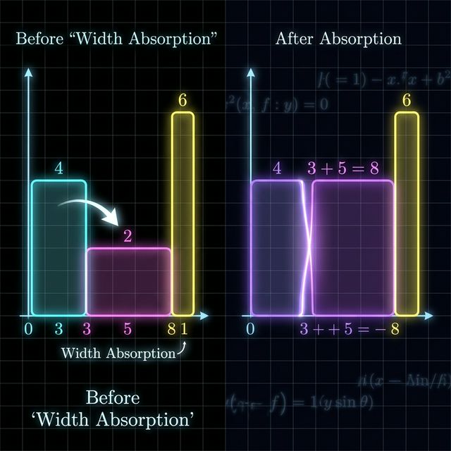
Here's the key modification: when a taller bar gets popped by a shorter bar, don't just discard the popped bar's width. Instead, accumulate it. The shorter bar "absorbs" the width of everything it eclipses.

Why does this work? Think about what happens in the standard algorithm. When bar i pops bar j (because bar i is shorter), bar i's height extends backward through bar j's entire range. In the unit-width version, this is implicit -- the width calculation i - left - 1 captures it. In the weighted version, we need to track it explicitly.

The accumulated width is the answer to: "how far back does the current bar's height extend?"

Walkthrough

Let's trace through bars = [(4, 3), (2, 5), (6, 1), (1, 2)].

Bar (4, 3) arrives. Stack is empty. Push it.

Stack: [(4, 3)]

Bar (2, 5) arrives. Height 2 < 4, so pop (4, 3). Rectangle: 4 * 3 = 12. The width 3 doesn't vanish -- it gets added to the incoming bar's effective width because height 2 extends back through everything we just popped. Push (2, 5 + 3 = 8).

Stack: [(2, 8)]

Bar (6, 1) arrives. Height 6 > 2, so nothing gets popped. Push it.

Stack: [(2, 8), (6, 1)]

Bar (1, 2) arrives. Height 1 < 6, so pop (6, 1). Rectangle: 6 * 1 = 6. Accumulated width: 1. Still going -- height 1 < 2, so pop (2, 8). Rectangle: 2 * (8 + 1) = 18. Accumulated width: 8 + 1 = 9. Now the stack is empty. Push (1, 2 + 9 = 11).

Stack: [(1, 11)]

End of input. Flush the stack with a sentinel of height 0. Pop (1, 11). Rectangle: 1 * 11 = 11.

Maximum rectangle: 18. That's the bar of height 2 stretching across a combined width of 9 -- its own width of 5 plus the 3 it absorbed from the popped bar of height 4.

What Just Happened

The width accumulation IS the state compression. In the expanded version, we'd have 3 + 5 + 1 + 2 = 11 unit bars and the stack would process each one individually. In the compressed version, we processed exactly 4 bars -- one per distinct entry.

Every time we pop a bar, we add its width to a running total. Every time we push a bar, its effective width includes everything it absorbed. This maintains the invariant that each stack entry knows exactly how far back its height extends.

Complexity

The standard histogram algorithm is O(N) where N is the number of unit-width bars. The weighted version is O(B) where B is the number of distinct bars, regardless of the total width.

Each bar is pushed once and popped once. That's 2B stack operations total. The total width could be 10^9 or 10^18 -- it doesn't matter. You never expand it.

Where This Shows Up

Coordinate compression problems. You have events at positions scattered across a huge range (say, 0 to 10^9), but there are only 10^5 distinct positions. The gaps between positions become bar widths.

Frequency-based histograms. Count character frequencies in a string: each character has a count that acts as a bar width. If you sort by height and treat each group as a weighted bar, you can find the largest rectangle in the frequency histogram without expanding.

Sparse data over large domains. Any time the problem says "coordinates up to 10^9" but "at most 10^5 events," you're probably looking at a weighted histogram in disguise.

The Pattern

This lesson adds one idea to your toolkit: when bars have non-unit widths, accumulate width on pop instead of computing it from index differences. Everything else -- the monotonic stack, the pop-when-shorter invariant, the sentinel flush -- stays exactly the same.

The standard algorithm implicitly tracks width through index arithmetic. The weighted algorithm explicitly tracks width through accumulation. Same logic, different bookkeeping. Once you see the connection, switching between the two is mechanical.

Tying It Back

This chapter started with the observation that every array is a histogram. Lesson 2 gave you the rectangle algorithm for unit-width bars. Lesson 3 showed you the contribution technique. Lesson 4 extended everything to 2D matrices.

This lesson removes the last restriction: bars don't need to have the same width. With weighted histograms, you can handle compressed coordinates, sparse domains, and frequency tables -- all with the same monotonic stack, running in time proportional to the number of distinct bars rather than the total width of the domain.