Greedoids, Matroids, and When Greedy Works
Every greedy algorithm you've used in this course works for a mathematical reason. This lesson reveals that reason.
Throughout Chapters 1-9, we built intuition for when greedy works: exchange arguments, stays-ahead proofs, structural properties. But underneath every one of those arguments lies a common mathematical framework. The theory of greedoids and matroids gives us a single lens to see why Kruskal's algorithm, Dijkstra's algorithm, interval scheduling, and Huffman coding all succeed — and why greedy fails spectacularly on knapsack or non-canonical coin systems.
This lesson is pure theory. There is no problem to solve. The goal is to connect every chapter of this course to a unified mathematical foundation.
1. The Generic Greedy Algorithm
Before defining any structures, let's pin down what "greedy" means in the abstract. Given a finite ground set \(S\) of elements, a weight function \(w : S \to \mathbb{R}\), and a notion of "feasibility," the generic greedy algorithm is:
- Sort elements of \(S\) by decreasing weight.
- Initialize the chosen set \(F = \emptyset\).
- For each element \(s\) in sorted order: if \(F \cup \{s\}\) is feasible, add \(s\) to \(F\).
- Return \(F\).
The Greedy Choice: At every step, pick the highest-weight element that keeps the solution feasible.
The snippet above implements this directly. The entire question of greedy correctness reduces to: for which definitions of "feasible" does this procedure find the optimum?
2. Greedoids: The Minimal Structure for Greedy
A greedoid is a pair \((S, \mathcal{F})\) where \(S\) is a finite ground set and \(\mathcal{F} \subseteq 2^S\) is a collection of feasible sets satisfying two axioms.
Axiom 1 (Accessibility):
The empty set is always feasible. You can always start from nothing.
Axiom 2 (Exchange Property):
In plain English: you can always grow a small feasible set toward a big one, one element at a time.
These two axioms are surprisingly powerful. Axiom 2 is the reason greedy "makes progress" — at every step, you're guaranteed that extending your current solution is possible. Without it, you could get stuck with a feasible set that cannot grow, even though larger feasible sets exist.
Why "greedoid"?
The name is a portmanteau of "greedy" and "matroid." Korte and Lovász introduced greedoids in 1981 specifically to characterize the structures on which greedy algorithms have good behavior. The idea was to find the weakest possible axioms that still let greedy work.
A non-example
Consider the problem: "select a maximum-weight subset of integers from \(\{1, 2, \ldots, n\}\) such that no two selected integers are adjacent." The feasible sets are independent sets in a path graph. Does this form a greedoid?
Take \(A = \{1, 4\}\) and \(B = \{3\}\). We have \(|A| > |B|\). But \(B \cup \{1\} = \{1, 3\}\) has two adjacent elements (not feasible), and \(B \cup \{4\} = \{3, 4\}\) also has adjacent elements (not feasible). The exchange property fails. This is not a greedoid, which is exactly why greedy fails on maximum-weight independent set in general graphs.
3. Matroids: Greedoids with Downward Closure
A matroid is a greedoid \((S, \mathcal{F})\) with one additional axiom:
Axiom 3 (Downward Closure / Hereditary Property):
Every subset of a feasible set is feasible. This is also called the hereditary property. Matroids are the "nicest" greedoids — they have the strongest structure.
The key theorem, due to Rado (1957) and Edmonds (1971):
Theorem (Rado-Edmonds). The generic greedy algorithm finds a maximum-weight feasible set for every weight function \(w : S \to \mathbb{R}\) if and only if \((S, \mathcal{F})\) is a matroid.
This is a remarkable characterization. Matroids are not just sufficient for greedy optimality — they are necessary. If your feasible sets don't form a matroid, there exists some weight function where greedy fails.
Classical matroid examples
Graphic matroid (forests in a graph). Let \(S\) = edges of graph \(G\), and \(\mathcal{F}\) = all acyclic subsets (forests). Any subset of a forest is a forest, so downward closure holds. The exchange property holds because a forest with more edges has more components joined, and you can always find an edge to add to a smaller forest. Kruskal's algorithm optimizes over this matroid.
Vector matroid (linear independence). Let \(S\) = a set of vectors in \(\mathbb{R}^d\), and \(\mathcal{F}\) = all linearly independent subsets. Subsets of independent sets are independent (downward closure). The Steinitz exchange lemma gives the exchange property.
Transversal matroid (matchings). Let \(S\) = elements on one side of a bipartite graph, and \(\mathcal{F}\) = subsets that can be matched to distinct neighbors. This satisfies both axioms.
Uniform matroid \(U_{k,n}\). Let \(S\) be any \(n\)-element set, and \(\mathcal{F} = \{A \subseteq S : |A| \le k\}\). Every subset of size at most \(k\) is feasible. Greedy on this matroid just picks the \(k\) heaviest elements — which is obviously optimal.
4. The Hierarchy: Which Algorithms Use Which Structures
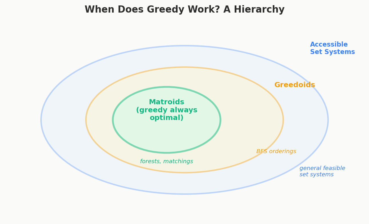
Not every greedy algorithm needs a full matroid. Some only need the weaker greedoid axioms. Here is how the algorithms from this course fit into the hierarchy:
| Algorithm | Structure | Type | Why greedy works |
|---|---|---|---|
| Kruskal's MST | Graphic matroid | Matroid | Exchange property + downward closure |
| Prim's MST | Undirected branching greedoid | Local forest greedoid | Exchange property (no downward closure needed) |
| Dijkstra | Directed branching greedoid | Local forest greedoid | Monotone path weights |
| Huffman | Merge-based construction | Matroid-like | Exchange argument on sibling depths |
| BFS | Point search antimatroid | Antimatroid | Upward closure |
| Interval scheduling | Interval greedoid | Matroid | Exchange on non-overlapping sets |
| Fractional knapsack | Uniform-like | Matroid | Items are continuously divisible |
The hierarchy from strongest to weakest:
Matroids give the strongest guarantees (greedy works for ALL weight functions). Greedoids give weaker guarantees (greedy works for SOME weight functions, under additional conditions on the weights). General accessible set systems give almost no guarantees.
Reading the table
A few things to notice:
- Kruskal's and Prim's solve the same problem (MST) but sit in different rows. Kruskal's has the full matroid guarantee; Prim's only has the greedoid guarantee. Both happen to find the correct answer because MST edge weights satisfy the extra conditions needed for greedoid optimality.
- Dijkstra is structurally similar to Prim's — both build rooted trees greedily. The key difference is that Dijkstra operates on a directed branching greedoid and requires non-negative edge weights to satisfy the optimality conditions.
- BFS lands in the antimatroid column, which is a fundamentally different structure. Antimatroids have upward closure instead of downward closure — they're in some sense "dual" to matroids.
- Huffman coding doesn't fit neatly into the matroid/greedoid hierarchy because it builds structure bottom-up (merging nodes) rather than top-down (selecting elements). But the exchange argument used to prove its optimality has the same flavor as matroid exchange.
5. Why Prim's Algorithm Is NOT a Matroid
This is a crucial distinction that many textbooks gloss over. Kruskal's and Prim's both find MSTs, but they operate on fundamentally different structures.
Kruskal's operates on the graphic matroid: feasible sets are forests (acyclic edge subsets). This is a matroid because every subset of a forest is a forest.
Prim's operates on a different structure. A feasible set for Prim's is a set of edges that forms a connected subtree rooted at the starting vertex. Let's see why this is not a matroid.
Concrete counterexample
Consider a path graph: \(A - B - C - D\), with Prim starting at vertex \(A\).
The edge set \(\{A\text{-}B,\; B\text{-}C,\; C\text{-}D\}\) is feasible — it's a connected subtree from \(A\).
Now remove the middle edge \(B\text{-}C\). The remaining set \(\{A\text{-}B,\; C\text{-}D\}\) is not feasible. The edge \(C\text{-}D\) is disconnected from \(A\). You can't reach \(C\) without going through \(B\text{-}C\) first.
So we have a feasible set whose subset is not feasible. Downward closure fails. Prim's structure is not a matroid.
But it is a greedoid. The exchange property still holds: given any two connected subtrees from the root, the larger one always contains an edge that can extend the smaller one (by taking an edge incident to the frontier of the smaller tree). This is a local forest greedoid, also called a branching greedoid.
The Greedy Choice: Prim's algorithm works not because forests form a matroid, but because connected subtrees from a root form a greedoid. The exchange property is enough.
This explains something subtle: Kruskal's finds the MST regardless of which edge you break ties with (matroid guarantees optimality for all weight functions). Prim's finds the MST too, but the intermediate feasible sets are more constrained — you must always maintain connectivity to the root.
6. The Greedy Optimality Theorem
When does greedy find the optimum on a greedoid that isn't a matroid? The answer requires conditions on the weight function, not just the combinatorial structure.
Theorem (Greedy Optimality on Greedoids). Let \((S, \mathcal{F})\) be a greedoid and \(w : S \to \mathbb{R}\) a weight function. The greedy algorithm finds a maximum-weight maximal feasible set if the following two conditions hold:
Condition 1 (Optimality is persistent): If element \(x\) is the best choice to extend feasible set \(F\), and \(F\) can be extended to a larger feasible set \(F'\) that also contains \(x\), then \(x\) is still a valid greedy choice at the point where it's added in \(F'\).
Condition 2 (Early selection doesn't hurt): Picking element \(x\) at step \(i\) produces a result at least as good as picking \(x\) at any later step \(j > i\).
In plain English: the best choice now stays the best choice later, and acting early doesn't hurt.
For matroids, both conditions hold automatically for any weight function — that's the content of the Rado-Edmonds theorem. For non-matroid greedoids, you must verify these conditions for your specific weight function.
Why Dijkstra satisfies this theorem
Dijkstra's algorithm operates on a directed branching greedoid (shortest-path trees from a source). The weight function is \(w(v) = -d(s, v)\), the negative of the shortest-path distance (we maximize negative distance, i.e., minimize distance).
- Condition 1: If vertex \(v\) has the smallest tentative distance when we process it, this distance is final (it can't decrease later, because all edge weights are non-negative). Optimality persists.
- Condition 2: Processing \(v\) early only helps — it lets us relax \(v\)'s outgoing edges sooner, potentially reducing tentative distances for other vertices.
This is precisely why Dijkstra fails with negative edge weights: Condition 1 breaks. A vertex processed early might later find a shorter path through a negative-weight edge, meaning its "optimal" choice at step \(i\) was not actually optimal.
7. Antimatroids: The Dual Side
An antimatroid is, roughly speaking, the "complement" of a matroid. Where matroids have downward closure (subsets of feasible sets are feasible), antimatroids have upward closure: supersets of feasible sets are feasible (up to the ground set).
More precisely, an antimatroid is a greedoid \((S, \mathcal{F})\) where:
Feasible sets are closed under union.
BFS as an antimatroid. Consider BFS from a source vertex \(s\). The feasible sets are "BFS layers" — sets of vertices reachable within some number of hops. If you can reach vertex set \(A\) and vertex set \(B\) via BFS, you can certainly reach \(A \cup B\). The structure is an antimatroid (specifically, a point search antimatroid).
This is why BFS correctly finds shortest paths in unweighted graphs, but the reason is structurally different from why Dijkstra works. BFS exploits upward closure; Dijkstra exploits the greedoid exchange property with monotone weights.
8. When Greedy MUST Fail
The theory gives us a clean way to explain greedy failures. If the feasible sets don't form a greedoid, greedy has no structural reason to work.
Non-canonical coin systems
Consider coins \(\{1, 3, 4\}\) and target sum \(6\). Greedy picks \(4 + 1 + 1 = 3\) coins. Optimal is \(3 + 3 = 2\) coins.
The "feasible sets" here are multisets of coins summing to at most the target. Does the exchange property hold? Take \(A = \{3, 3\}\) (sum 6) and \(B = \{4\}\) (sum 4). We have \(|A| > |B|\). But \(B \cup \{3\} = \{4, 3\}\) sums to 7, which exceeds the target — not feasible. The exchange property fails. Not a greedoid.
For the canonical system \(\{1, 5, 10, 25\}\), the exchange property does hold (this is non-trivial to prove and specific to the denomination structure). The coin system forms a matroid-like structure, and greedy works.
0/1 Knapsack
Items have weights and values. Feasible sets are subsets with total weight \(\le W\). This forms a matroid (it's actually an instance of the uniform-matroid generalization). But the objective is not a modular function — the value of a set isn't determined by individual element weights in the matroid sense. The greedy weight ordering (value/weight ratio) does not align with the matroid structure. Greedy finds the optimum for fractional knapsack (where items are divisible) but not for 0/1 knapsack.
Maximum-weight independent set
As shown in Section 2, independent sets on general graphs violate the exchange property entirely. This is why maximum-weight independent set is NP-hard — there is no greedoid structure to exploit.
The pattern
In every failing case, the diagnosis is the same: either the exchange property breaks (coins, independent set) or the weight function doesn't respect the greedoid structure (0/1 knapsack). The theory doesn't just tell us that greedy fails — it tells us why, and it points to exactly which axiom or condition is violated. This is the real power of the framework: it turns vague intuition ("greedy seems wrong here") into a precise structural diagnosis.
9. The Ordered vs. Unordered Distinction
There is a subtle issue in the theory that was only recently resolved.
The generic greedy algorithm processes elements in a fixed order (sorted by weight). This is the ordered version. But some greedy algorithms, like Prim's, don't use a fixed global order — they make locally optimal choices that depend on the current state. This is the unordered version.
In the original 1981 paper, Korte and Lovász claimed that greedy optimality results for greedoids held in both the ordered and unordered cases. This claim was wrong.
In 2021, Szeszler published a correction showing that the unordered greedy is only guaranteed to work for a subclass called local forest greedoids. For general greedoids, the order in which you process elements can matter.
This distinction explains a practical phenomenon:
- Kruskal's (matroid, ordered): Sort all edges globally, process in order. The global ordering is essential and sufficient.
- Prim's (local forest greedoid, unordered): Pick the cheapest edge from the current frontier. The choice depends on state, not a precomputed order.
Both find the MST, but for different structural reasons. Prim's works because branching greedoids belong to the "local forest" subclass where unordered greedy is safe.
The Greedy Choice: The order of greedy decisions can matter. For matroids, any consistent ordering works. For general greedoids, only specific orderings are safe.
10. Connection to This Course
The greedoid/matroid framework gives a clean map of the entire course.
Chapters 1-4: Pure Greedy (Matroid and Greedoid Territory)
Every problem in these chapters succeeds because the underlying combinatorial structure is a matroid or greedoid:
- Chapter 1 (Greedy Mindset): Sorting-based greedy works because the problems have matroid-like structure. The "exchange" intuition from Chapter 1 is an informal version of Axiom 2.
- Chapter 2 (Exchange Arguments): Exchange arguments are proofs that the matroid exchange property holds. When you show "swapping two elements doesn't worsen the solution," you're verifying the exchange axiom.
- Chapter 3 (Stays Ahead): Stays-ahead proofs show that greedy's intermediate solutions dominate all alternatives — this is the Greedy Optimality Theorem in action.
- Chapter 4 (Structural Greedy): MST algorithms (Kruskal, Prim) directly exploit graphic matroids and branching greedoids.
Chapters 5-8: Beyond Greedoids
When the underlying structure is not a greedoid, pure greedy fails. But the problems in these chapters have a different kind of structure — concavity — that allows modified greedy approaches:
- Chapter 5 (Greedy + Undo): The structure isn't a greedoid (greedy can make mistakes), but the cost function is concave enough that undoing a bounded number of decisions recovers optimality.
- Chapter 7 (WQS / Lambda Optimization): The cost function \(f(k)\) is concave in the number of components \(k\). WQS exploits this by binary searching on a Lagrange multiplier \(\lambda\), converting a constrained problem into an unconstrained one where greedy (on the modified weights) works. The modified problem does have greedoid structure.
- Chapter 8 (Advanced Graph Greedy): Problems like Boruvka's and advanced MST variants use the matroid structure directly but with more sophisticated algorithms.
Chapter 9: Classic Problems
The classic problems revisited in Chapter 9 are a mix: some are pure matroids (activity selection), some are greedoids (Huffman), and some require careful structural arguments (scheduling with deadlines uses a transversal matroid).
11. Summary: The Structural Checklist
When you encounter a new problem and wonder "does greedy work?", here's the theoretical checklist:
Step 1. Define the ground set \(S\) and the collection of feasible sets \(\mathcal{F}\).
Step 2. Check the exchange property: if \(|A| > |B|\) for feasible \(A, B\), can you always find \(s \in A \setminus B\) with \(B \cup \{s\} \in \mathcal{F}\)?
- If no: not a greedoid. Greedy has no structural basis. Stop.
- If yes: proceed to Step 3.
Step 3. Check downward closure: is every subset of a feasible set also feasible?
- If yes: it's a matroid. Greedy works for every weight function. Done.
- If no: it's a greedoid but not a matroid. Proceed to Step 4.
Step 4. Check the two conditions of the Greedy Optimality Theorem:
- Does the best choice now remain the best choice later? (Persistence)
- Does choosing early never hurt? (Monotonicity)
If both hold for your specific weight function, greedy is optimal. Otherwise, greedy may fail even though the structure is a greedoid.
12. Historical Notes and Further Reading
The theory of matroids was introduced by Whitney in 1935, originally to abstract the notion of linear independence. Rado and Edmonds connected matroids to optimization in the 1950s-70s, proving the fundamental theorem that matroids exactly characterize when greedy works.
Greedoids were introduced by Korte and Lovász in 1981 as a generalization. Their original paper claimed certain results about unordered greedy that turned out to be incorrect — Szeszler's 2021 correction clarified that unordered greedy only works for local forest greedoids.
For a thorough modern treatment, see nor's excellent blog post: Greedoids - nor-blog
The key takeaway for competitive programmers: you don't need to formally verify matroid axioms during a contest. But understanding why greedy works — at the level of exchange properties and feasible sets — will sharpen your intuition for when to attempt a greedy approach and when to look for DP or other techniques.
Recommended reading path
If this lesson sparked your interest, here is a suggested order for deeper study:
- nor's blog post (linked above) — accessible, concrete, and oriented toward competitive programming.
- Oxley, "Matroid Theory" (2011) — the standard graduate textbook on matroids. Chapters 1-2 cover the fundamentals.
- Korte, Lovász, Schrader, "Greedoids" (1991) — the definitive monograph on greedoid theory. Dense but complete.
- Szeszler, "A note on greedy algorithms for greedoids" (2021) — the correction to the ordered/unordered distinction. Short and self-contained.
Key Takeaways
-
A greedoid is defined by two axioms: the empty set is feasible, and the exchange property holds. These are the minimal conditions for greedy to have a chance.
-
A matroid is a greedoid with downward closure. On a matroid, greedy is optimal for every weight function — this is the strongest guarantee.
-
Kruskal's operates on a matroid; Prim's operates on a greedoid that is not a matroid. Both find MSTs, but for different structural reasons.
-
On a non-matroid greedoid, greedy requires additional conditions on the weight function: optimality must persist, and early selection must not hurt.
-
When the exchange property fails entirely (knapsack, non-canonical coins, independent set), greedy has no mathematical basis and will fail for some inputs.
-
The order of greedy decisions matters for general greedoids but not for matroids or local forest greedoids.
-
Chapters 1-4 of this course live in matroid/greedoid territory. Chapters 5-8 handle problems outside this territory using concavity-based techniques.