Optimize Before You Scale

Optimize Before You Scale

TL;DR

Before you reach for replicas, caches, or CDNs, exhaust what your existing database can do. Proper indexing, smart denormalization, and better hardware solve 80% of read scaling problems — with zero operational complexity added.

Most engineers jump straight to "add a cache" or "spin up read replicas" the moment queries slow down. That's like buying a second car because your first one needs an oil change. The boring optimizations — indexes, denormalization, vertical scaling — are cheaper, simpler, and often all you need.

---

Indexing: The Single Biggest Read Optimization

An index is a sorted lookup structure that sits alongside your table. Instead of scanning every row to find what you need (O(n)), the database walks a tree to find it in O(log n).

The book analogy: You're looking for "replication lag" in a 500-page textbook. You don't flip through every page — you check the index at the back, find the page number, and jump there. A database index works the same way.

Index Types

Index Type	How It Works	Best For
B-tree	Balanced tree, sorted keys	Range queries, ordering, most workloads
Hash	Hash table, O(1) exact lookup	Exact match only (WHERE id = 42)
Full-text	Inverted index of words/tokens	Search queries (LIKE '%keyword%')
Composite	B-tree on multiple columns	Multi-column WHERE clauses

B-tree is the default in PostgreSQL, MySQL, and most databases. If someone says "index" without qualifying it, they mean B-tree.

See the Difference

Here's a query on an orders table with 10 million rows — first without an index, then with one:

-- Without index: full table scan
EXPLAIN ANALYZE
SELECT * FROM orders WHERE customer_id = 12345;

-- Result:
-- Seq Scan on orders  (cost=0.00..285432.00 rows=50 width=120)
--   Filter: (customer_id = 12345)
--   Rows Removed by Filter: 9999950
--   Execution Time: 1842.531 ms

-- Add the index
CREATE INDEX idx_orders_customer_id ON orders (customer_id);

-- With index: B-tree lookup
EXPLAIN ANALYZE
SELECT * FROM orders WHERE customer_id = 12345;

-- Result:
-- Index Scan using idx_orders_customer_id on orders
--   (cost=0.43..52.18 rows=50 width=120)
--   Index Cond: (customer_id = 12345)
--   Execution Time: 0.284 ms

That's a 6,500x speedup from a single CREATE INDEX statement. The query went from scanning 10 million rows to walking a tree and touching 50.

Under-indexing kills more apps than over-indexing

Engineers often fear adding "too many indexes" because they've heard indexes slow down writes. This is technically true — every INSERT must update every index. But in practice, the write overhead of an index is usually microseconds. Meanwhile, a missing index on a hot read path can bring your entire database to its knees. When in doubt, add the index. You can always drop it later.

When NOT to Index

Indexes aren't free. Skip them when:

• Columns you never filter or sort on. An index nobody queries is just wasted disk space.
• Tiny tables (< 1,000 rows). A full table scan on a small table is faster than the overhead of an index lookup.
• Write-heavy columns with few reads. If a column gets updated on every request but rarely queried, the index maintenance cost isn't worth it.

Deep Dive

B-tree internals, composite index ordering, and covering indexes are covered in depth in the Data Modelling course. This lesson covers indexing as a scaling strategy — that course covers it as a data modelling skill.

---

Denormalization: Trading Write Complexity for Read Speed

Normalization keeps your data clean — no duplicates, no anomalies, everything in its right place. But normalized schemas often require expensive JOINs to answer simple questions.

Denormalization is the deliberate decision to store redundant data so that reads can hit a single table instead of joining four.

The Normalized Version

Say you want to show an order summary page. In a fully normalized schema:

-- 4-table JOIN to build an order summary
SELECT
    o.id            AS order_id,
    o.created_at,
    o.status,
    c.name          AS customer_name,
    c.email         AS customer_email,
    p.name          AS product_name,
    p.price,
    oi.quantity,
    (p.price * oi.quantity) AS line_total
FROM orders o
JOIN customers c     ON c.id = o.customer_id
JOIN order_items oi  ON oi.order_id = o.id
JOIN products p      ON p.id = oi.product_id
WHERE o.id = 98765;

Four tables, three JOINs. Each JOIN is a potential performance cliff — especially when tables grow to millions of rows.

The Denormalized Version

Store the data you need for the read path directly on the order_summaries table:

-- Single table read — no JOINs
SELECT
    order_id,
    created_at,
    status,
    customer_name,
    customer_email,
    product_name,
    price,
    quantity,
    line_total
FROM order_summaries
WHERE order_id = 98765;

One table, zero JOINs, sub-millisecond response. But you're now responsible for keeping customer_name, product_name, and price in sync whenever the source data changes.

The Trade-Off

Factor	Normalized	Denormalized
Read speed	Slower (JOINs)	Faster (single table)
Write speed	Faster (one place to update)	Slower (must update copies)
Storage	Minimal	Redundant data uses more disk
Consistency	Strong (single source of truth)	Risk of stale copies
Schema changes	Easier	Harder (more places to update)
Query complexity	Complex reads, simple writes	Simple reads, complex writes

Materialized Views: The Middle Ground

A materialized view is a precomputed query result stored as a table. You get the read speed of denormalization without manually maintaining redundant columns — the database does it for you (on refresh).

-- Create a materialized view for average product ratings
CREATE MATERIALIZED VIEW product_ratings_summary AS
SELECT
    p.id          AS product_id,
    p.name        AS product_name,
    COUNT(r.id)   AS review_count,
    ROUND(AVG(r.rating), 2) AS avg_rating
FROM products p
LEFT JOIN reviews r ON r.product_id = p.id
GROUP BY p.id, p.name;

-- Query it like a regular table — instant response
SELECT product_name, avg_rating, review_count
FROM product_ratings_summary
WHERE avg_rating >= 4.0
ORDER BY review_count DESC
LIMIT 20;

-- Refresh it periodically (e.g., every hour via cron)
REFRESH MATERIALIZED VIEW CONCURRENTLY product_ratings_summary;

The CONCURRENTLY keyword lets the view refresh without blocking reads — critical for production use.

Denormalization is a Measured Decision, Not a Default

Denormalization creates a maintenance nightmare if you're not careful. Before you denormalize, measure. Run EXPLAIN ANALYZE on the slow query. Try adding indexes first. Only denormalize when you've proven the JOIN is actually the bottleneck — not because you assume it will be.

Interview Move

In system design interviews, mention denormalization as an optimization you'd apply after measuring, not as your default schema design. This shows you understand trade-offs and don't prematurely sacrifice data integrity.

---

Hardware: The Underrated Vertical Scaling

Before you add distributed infrastructure, ask: "Can I just throw money at the problem?"

Vertical scaling — upgrading the machine your database runs on — is the simplest scaling strategy. No code changes, no architectural complexity, no distributed systems headaches.

What Actually Matters

SSDs vs HDDs. Databases do enormous amounts of random I/O. SSDs are 10-100x faster at random reads than spinning disks. If your database is still on HDDs, switching to SSDs is the single highest-ROI hardware change you can make.

More RAM. Databases cache frequently accessed data in memory (the "buffer pool" in MySQL, "shared buffers" in PostgreSQL). The more RAM you give it, the more of your dataset lives in memory, and the fewer disk reads you need. If your working set fits entirely in RAM, reads become memory lookups instead of disk I/O.

Better CPU. More cores = more concurrent queries processed. Faster clock speed = faster individual query execution. This matters most for complex analytical queries.

The Numbers

Storage Tier	Random Read Latency	Relative Speed
HDD (spinning disk)	~10 ms	1x
SSD (SATA)	~0.1 ms	100x
NVMe SSD	~0.01 ms	1,000x
RAM	~100 ns (0.0001 ms)	100,000x

The gap between HDD and RAM is five orders of magnitude. Moving your hot data from disk to memory isn't an optimization — it's a category change.

Interview Tip

Mention vertical scaling first in an interview. It shows you don't prematurely add complexity. But don't dwell on it — interviewers usually want to hear about distributed solutions. Say something like: "First, I'd make sure we've exhausted vertical scaling — SSDs, more RAM, proper indexing. But assuming we're past that, here's how I'd scale horizontally..."

---

The Optimization Checklist

Before you move to Lesson 3 (read replicas) or Lesson 4 (caching), walk through this decision tree:

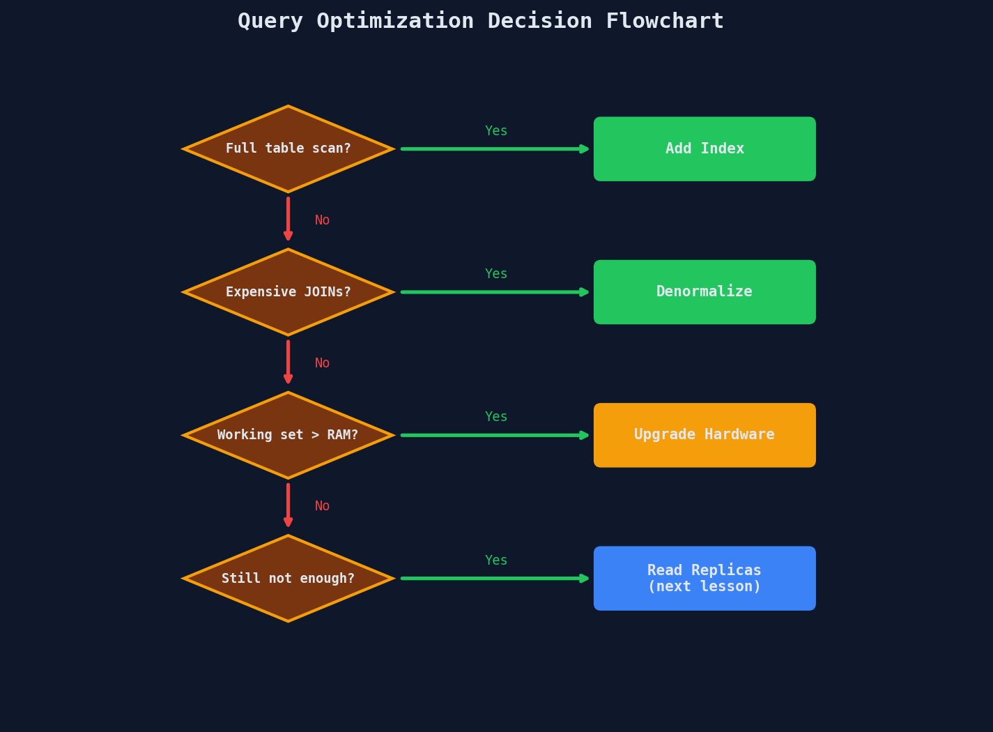
The key insight: each step in this flowchart is cheaper and simpler than the next lesson's solutions. An index costs nothing to operate. A materialized view is one SQL statement. A RAM upgrade is a cloud console slider. Read replicas, caches, and CDNs all require ongoing operational work — replication lag handling, cache invalidation, cache warming, consistency protocols.

Exhaust the cheap stuff first. Then scale.

---

What's Next

You've squeezed everything you can out of a single database instance. The queries are indexed, the hot JOINs are denormalized, and you're running on NVMe with 256 GB of RAM.

It's still not enough. Traffic keeps growing.

Time to make copies. Lesson 3: Read Replicas — how to distribute reads across multiple database instances, and the consistency headaches that come with it.