Properties & RMQ Equivalence
The Cartesian Tree isn't just a cute construction. It has three properties that make it genuinely useful, and together they connect range queries to tree structure in a tight, two-way relationship.
Property 1: Heap Order
The Cartesian Tree is a min-heap. Every node's value is less than or equal to every value in its subtree.
This follows directly from the construction. The root of any subtree is the minimum of the corresponding subarray. So a node's value is always the smallest in its subtree. That's the heap property.
For a max-Cartesian Tree, it's a max-heap instead. Same idea, flipped.
This is straightforward, but it matters. It means you can reason about the tree using heap intuition. Smaller values sit closer to the root. The global minimum is always at the root. If you want to know which elements "dominate" a range, just look at the ancestors.
Property 2: Inorder Completeness
An inorder traversal of the Cartesian Tree gives back the original array, in order. Index 0 first, then index 1, then index 2, all the way through.
Why? Because of how we split. The root is some index m. Everything with index less than m is in the left subtree. Everything with index greater than m is in the right subtree. An inorder traversal visits the left subtree (indices < m), then the root (index m), then the right subtree (indices > m). Recursively, this produces the original ordering.
The important consequence: each subtree corresponds to a contiguous subarray. The subtree rooted at node u covers some range [l, r] of the original array, and every index in that range is in the subtree — no gaps, no extras.
This is what makes the Cartesian Tree different from a regular heap. A regular heap doesn't preserve array order. The Cartesian Tree preserves it perfectly.
Think of it this way: the tree is simultaneously sorted by value (vertically, via the heap property) and sorted by index (horizontally, via the inorder property). It encodes both orderings at once.
Property 3: LCA = RMQ
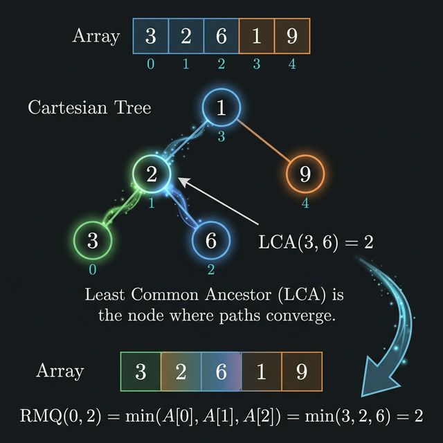
This is the big one. The Lowest Common Ancestor of nodes i and j in the Cartesian Tree is the minimum element in A[i..j].
Let's prove it. Take two indices i < j. Their LCA is the deepest node that has both i and j in its subtree. Since each subtree is a contiguous range (Property 2), the LCA's range is the smallest contiguous range containing both i and j. That range is [i..j] itself (or some range containing it). And the root of that subtree is the minimum of its range (Property 1).
More precisely: the LCA's range [l, r] must satisfy l <= i and r >= j. The LCA is the deepest such node, meaning [l, r] is as small as possible. The smallest contiguous range containing both i and j is [i, j]. And the root of the subtree for range [i, j] is argmin(A[i..j]).
So LCA(i, j) = argmin(A[i..j]).
This is a two-way equivalence:
- Range minimum queries reduce to LCA queries on the Cartesian Tree.
- LCA queries reduce to range minimum queries on the original array (using the Euler tour technique, but that's a different story).
In practice, this means if you have a Cartesian Tree with an LCA structure (binary lifting, or Euler tour + sparse table), you can answer range minimum queries in O(log N) or even O(1) per query.
The Ancestor Chain
Here's a corollary that shows up in problems more often than you'd expect.
Pick any node i in the Cartesian Tree. Now walk from i up to the root, collecting every ancestor along the way. What do you get?
Each ancestor is the root of a progressively larger subtree, which means it's the minimum of a progressively wider range. And since we're going up the tree, each ancestor has a smaller value than the one below it (heap property).
So the path from node i to the root gives you all elements that are the minimum of some range containing i, listed in decreasing order of their values.
Think of it as a sequence of "dominant" elements. The parent of i dominates a slightly wider range. The grandparent dominates an even wider range. Each ancestor "sees" further than the one below it.
This means: the depth of node i tells you how many elements dominate progressively wider ranges containing i. Deep nodes are hemmed in by many smaller elements nearby. Shallow nodes near the root are the ones doing the dominating.
Why This Matters in Practice
You might wonder: if I just want range minimum queries, I can use a sparse table and get O(1) per query without building a tree. Why bother with the Cartesian Tree?
Fair point. For pure RMQ, a sparse table is simpler. The Cartesian Tree becomes useful when you need both range minimum queries and structural reasoning about the tree.
Here are situations where the tree structure helps:
-
Subtree sizes. The size of node
i's subtree tells you the length of the range it dominates. You can compute this in O(N) with a single DFS. -
Parent-child relationships. Knowing that
jis the parent ofitells you thata[j]is the minimum of some range that strictly containsi's range. You don't need any queries to know this — it's baked into the structure. -
Tree DP. When a problem asks you to compute something over all subarrays based on their minimums, you can do a DP over the Cartesian Tree. Each node decides for its range, and the left/right children handle the sub-ranges. We'll see this in the next lesson.
-
Decomposition. The Cartesian Tree gives you a natural divide-and-conquer decomposition of the array. The root splits the array at the global minimum, and each half is handled recursively. This is often cleaner than iterating over subarrays directly.
The short version: the Cartesian Tree is the bridge between "flat" array problems and "tree" algorithms. Whenever you find yourself needing to reason about minimums across ranges and also need tree structure, the Cartesian Tree is probably the right tool.
Connection to the Contribution Technique
Remember the contribution technique from Chapter 3? For each element, you computed how many subarrays it was the minimum of, using left and right boundaries.
Those boundaries are exactly the parent-child relationships in the Cartesian Tree. The left boundary of element i is determined by its nearest smaller element to the left — which is its closest ancestor reached by going up from a left-child link. The right boundary is similar.
The contribution of element i is a[i] * left_count * right_count, where left_count and right_count depend on the shape of i's subtree and where i sits relative to its parent.
You were doing tree computations in Chapter 3 without knowing the tree existed. Now you can see the structure explicitly, and in the next lesson, you'll use it to solve problems that the contribution technique alone can't handle.
Verifying Your Tree
A good sanity check after building a Cartesian Tree: run an inorder traversal and verify you get indices 0, 1, 2, ..., n-1 in order. If you don't, something's wrong with the construction. The "Inorder Verification" snippet does exactly this.
Another check: for every node u with children l and r, verify that a[u] <= a[l] and a[u] <= a[r]. That confirms the heap property.
Try It
The starter code builds the Cartesian Tree and sets up binary lifting for LCA queries. You need to fill in the LCA function and answer range minimum queries.
Test with:
Expected output:
Query (0, 4): minimum of entire array is 1 at index 3.
Query (0, 2): minimum of [3, 2, 6] is 2 at index 1.
Query (2, 4): minimum of [6, 1, 9] is 1 at index 3.
Each answer is the index returned by the LCA — and that index holds the minimum value in the queried range.