Matrix Elevations — 2D Histograms
From 1D to 2D
You can solve Largest Rectangle in Histogram in O(N). Great. Now here's a harder problem: given a binary matrix (all 0s and 1s), find the largest rectangle containing only 1s.
This is LeetCode 85 (Maximal Rectangle). It looks like a different beast — a 2D problem, not a histogram problem. But here's the trick that makes it fall: every row of the matrix is the base of a histogram.
Once you see that, the 2D problem becomes N applications of the 1D problem. And you already know how to solve the 1D problem.
The Height Array
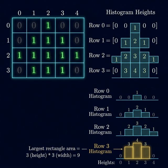
Take this 4x5 binary matrix:
For each cell, ask: "How many consecutive 1s are stacked above this cell, including itself?" That gives you the height of each cell.
The rule is simple:
- If
grid[i][j] == 0, thenheight[j] = 0(the streak is broken). - If
grid[i][j] == 1, thenheight[j] = height[j] + 1(the streak continues from the previous row).
Let's compute the heights row by row.
Row 0 — This is the first row, so heights are just the row values:
Picture this as a histogram:
Largest rectangle in this histogram: 1.
Row 1 — For each column, if the current cell is 1, add 1 to the previous height. If it's 0, reset to 0.
The histogram:
Largest rectangle: let's check. Bar 0 (height 2): L=−1, R=1, width=1, area=2. Bar 2 (height 2): L=1, R=3, width=1, area=2. Bar 3 (height 1): L=1, R=5, width=3, area=3. Bar 4 (height 1): L=1, R=5, width=3, area=3. Max = 3 (a 1x3 rectangle spanning columns 2-4).
Row 2 — Every cell in this row is 1, so every height increases:
The histogram:
This is where things get interesting. Let's compute the largest rectangle:
- Bar 0 (height 3): L=−1, R=1, width=1, area=3.
- Bar 1 (height 1): L=−1, R=5, width=5, area=5.
- Bar 2 (height 3): L=1, R=3, width=1, area=3.
- Bar 3 (height 2): L=1, R=5, width=3, area=6.
- Bar 4 (height 2): L=1, R=5, width=3, area=6.
Max = 6. That's a 2x3 rectangle (height 2, columns 2-4, rows 1-2). Check the original matrix — rows 1-2, columns 2-4: all 1s. Correct.
Row 3 — Some cells are 0, and this is where the height reset matters. Let's trace column by column:
| Column | grid[3][col] | Previous height | New height | Why? |
|---|---|---|---|---|
| 0 | 1 | 3 | 4 | Streak continues: 3 + 1 = 4 |
| 1 | 0 | 1 | 0 | A zero RESETS the height to 0. The streak of 1s above is irrelevant — there's a gap now. |
| 2 | 0 | 3 | 0 | Same thing. Column 2 had a height of 3, but the 0 kills it. |
| 3 | 1 | 2 | 3 | Streak continues: 2 + 1 = 3 |
| 4 | 0 | 2 | 0 | Reset. |
The 0-reset is the single most common source of bugs in this problem. Students often try to "subtract 1" or "carry forward" through a zero. Don't. A zero means the rectangle can't extend through this cell, period. Height goes to 0.
The histogram:
Largest rectangle: bar 0 has area 4 (4x1), bar 3 has area 3 (3x1). Max = 4.
Overall answer: the maximum across all rows is 6, found at row 2.
Why This Works
Think about what the height array represents. When heights[j] = 3 at row i, that means cells (i, j), (i-1, j), and (i-2, j) are all 1s. It's a column of three consecutive 1s ending at the current row.
Now when you run Largest Rectangle in Histogram on this height array, you're finding the widest rectangle of consecutive columns where all the heights are at least some value h. That rectangle corresponds to an h by w block in the original matrix where every cell is 1.
By processing every row as a separate histogram base, you're considering every possible position for the bottom edge of the rectangle. The top edge is determined by the heights. So you cover all possible rectangles.
The Algorithm
Here it is in full:
- Initialize
heights[0..M-1] = 0. - For each row
ifrom0toN-1: a. For each columnj, update: ifgrid[i][j] == 1, incrementheights[j]; else setheights[j] = 0. b. Run Largest Rectangle in Histogram onheights. Update the global max. - Output the global max.
The height update is O(M) per row. The histogram solve is O(M) per row. Over N rows, the total is O(N * M).
That's optimal — you can't even read the whole matrix faster than O(N * M).
Implementation Details
A few things to watch for when you code this up.
Reuse the heights array. Don't allocate a new array for each row. Just update in place. The whole point is that the height at column j carries forward from the previous row — you're building on it.
Use the single-pass histogram solution. Since you don't need the boundary arrays for anything else (no contribution counting here), the single-pass approach with the sentinel is cleaner. It processes the histogram in one scan and doesn't need extra arrays.
Watch for the matrix input format. Some problems give the matrix as characters ('0' and '1'), others as integers. Make sure you're parsing correctly. A common bug is reading '1' (ASCII 49) when you expected the integer 1.
Maximal Square vs. Maximal Rectangle
You might've seen the Maximal Square problem (LeetCode 221): find the largest square of all 1s. That one has a simpler DP solution — dp[i][j] = min(dp[i-1][j], dp[i][j-1], dp[i-1][j-1]) + 1 if grid[i][j] == 1.
The histogram method is more general. It finds rectangles of any aspect ratio, not just squares. The DP approach for squares is elegant but doesn't generalize. If you need rectangles, you need histograms.
That said, the DP approach for squares is O(N*M) too. So if the problem specifically asks for squares, use the DP. If it asks for rectangles, use the histogram method.
Extending the Pattern
The row-by-row histogram reduction isn't limited to "largest rectangle of all 1s." You can adapt it to:
- Largest rectangle where all values are the same — maintain a height array per distinct value, or reset height when the value changes from the previous row.
- Largest rectangle where all values are >= K — treat cells with value >= K as 1 and the rest as 0.
- Count of all-1 rectangles — instead of tracking just the max area, sum up contributions. Each bar's boundary pair defines how many rectangles include that bar as the constraint.
The key insight stays the same every time: reduce each row to a 1D histogram, then apply whatever 1D tool you need. The monotonic stack handles the 1D part in O(M), and you repeat for N rows.
Putting It All Together
This is the capstone of the histogram chapter. Let's recap the chain of ideas:
Lesson 1: Every array is a histogram. Each element has a range of dominance defined by its left and right boundaries. The monotonic stack computes these in O(N).
Lesson 2: The Largest Rectangle in Histogram problem is a direct application of boundaries. Each bar's max rectangle = height * (right boundary - left boundary - 1).
Lesson 3: The Contribution Technique flips the perspective. Instead of "what's the min of each subarray?", ask "how many subarrays is each element the min of?" Same boundaries, different formula.
Lesson 4 (this one): 2D matrix problems reduce to repeated 1D histogram problems. Build heights row by row, solve the 1D problem for each row.
All four lessons share the same core: the monotonic stack computes boundaries, and those boundaries power everything else. Whether you're computing areas, counting subarrays, or reducing 2D to 1D — the stack is doing the same thing every time. The problems look different on the surface, but they're all histograms underneath.