Heights & Boundaries

Every Array Is a Histogram

Here's a shift in perspective that'll change how you see monotonic stack problems.

Take any array — say [2, 1, 5, 6, 2, 3]. Now draw it. Index on the x-axis, value on the y-axis. Each element becomes a bar. You've got a histogram.

6       |
5     | |
4     | |
3     | |   |
2 |   | | | |
1 | |   | | |
  0 1 2 3 4 5

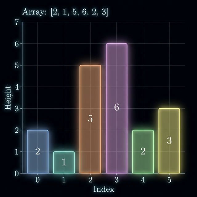
This isn't just a cute picture. It's a way of thinking. When you see an array as a collection of bars with different heights, new questions pop up naturally. How far does each bar "reach" before a shorter bar blocks it? What's the biggest rectangle you can fit under these bars? How many subarrays does a particular bar dominate?

All of these questions lead to the same underlying structure: boundaries.

Left Boundary and Right Boundary

Let's define two things for each element A[i]:

• Left boundary L[i]: the nearest index j < i where A[j] < A[i]. If nothing is smaller to the left, we say L[i] = -1.
• Right boundary R[i]: the nearest index j > i where A[j] < A[i]. If nothing is smaller to the right, we say R[i] = N.

Think of it this way. You're standing on bar i, looking left. The left boundary is the first bar that's shorter than you. Same idea looking right.

Between these two boundaries — from index L[i]+1 to R[i]-1 — bar i is the shortest bar. No bar in that range is shorter. It's the minimum of that subarray.

Wait. "Nearest index to the left where something is smaller." That's just Previous Smaller Element. And "nearest index to the right where something is smaller" is Next Smaller Element. You've already built both of these in Chapter 1. This is the same machinery, just with a new name and a geometric interpretation.

Walkthrough: [2, 1, 5, 6, 2, 3]

Let's compute boundaries for each element. We're looking for strictly smaller elements.

Index i	Value A[i]	Left Boundary L[i]	Right Boundary R[i]	Dominance Range
0	2	-1	1	[0, 0]
1	1	-1	6	[0, 5]
2	5	1	4	[2, 3]
3	6	2	4	[3, 3]
4	2	1	6	[2, 5]
5	3	4	6	[5, 5]

Let's trace a couple of these to make sure they click.

Index 2 (value 5): Looking left from index 2, the first element smaller than 5 is index 1 (value 1). So L[2] = 1. Looking right, the first element smaller than 5 is index 4 (value 2). So R[2] = 4. The dominance range is [L+1, R-1] = [2, 3]. Check: the subarray [5, 6] — yep, 5 is the minimum there.

Index 1 (value 1): Nothing to the left is smaller, so L[1] = -1. Nothing to the right is smaller either, so R[1] = 6 (which is N). Dominance range: [0, 5] — the entire array. Makes sense. 1 is the global minimum.

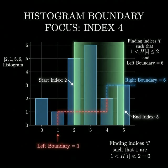
Index 4 (value 2): Left boundary is index 1 (value 1). Right boundary is 6 (nothing smaller to the right). Dominance range: [2, 5]. Subarray [5, 6, 2, 3] — and 2 is the minimum. Correct.

Range of Dominance

Let's give this concept a name. The range of dominance of element A[i] (with respect to minimum) is the contiguous subarray A[L[i]+1 .. R[i]-1] where A[i] is the minimum element.

Why is this useful? Two big reasons:

1. Rectangle problems. If A[i] is the shortest bar in the range [L[i]+1, R[i]-1], then the widest rectangle with height A[i] has width R[i] - L[i] - 1. Multiply height by width and you've got the area of the biggest rectangle constrained by bar i. We'll use this in the next lesson to solve Largest Rectangle in Histogram.

2. Contribution problems. If A[i] is the minimum of the subarray [L[i]+1, R[i]-1], then it's also the minimum of every subarray contained within that range that includes index i. How many such subarrays? That's a counting question, and it leads to the Contribution Technique in lesson 3.

Both of these categories collapse into the same two-step pattern:

1. Run the monotonic stack to compute left and right boundaries.
2. Use the boundaries for the actual computation (area, count, whatever).

Computing Boundaries with the Monotonic Stack

You know how to do this from Chapter 1, but let's write it out one more time in the boundary language.

Left boundaries — scan left to right. Maintain a stack of indices. For each i, pop everything from the stack that's >= A[i]. The top of the stack after popping is L[i]. If the stack is empty, L[i] = -1. Push i.

Right boundaries — scan right to left. Same logic, same stack discipline. For each i, pop everything >= A[i]. The top after popping is R[i]. If the stack is empty, R[i] = N. Push i.

Both passes are O(N). Each element is pushed once and popped at most once. Total: O(N) time, O(N) space.

A quick note: we used >= in the popping condition, which gives us strictly smaller boundaries. If you need less than or equal boundaries (useful for handling duplicates), you'd use > instead. We'll see exactly when this matters in the contribution technique lesson.

Flipping the Direction

Everything above was "range where A[i] is the minimum." You can do the exact same thing for maximum — just flip the comparison. Left boundary becomes the nearest element greater than A[i], and so on. The monotonic stack direction changes (you'd maintain an increasing stack instead of decreasing, or vice versa), but the logic is identical.

Don't memorize separate templates for min and max. Understand the one template, and flip the comparison operator when you need the other.

What's Coming Next

You now have a way to take any array, run two O(N) passes, and know each element's range of dominance. That's the foundation for everything in this chapter.

Next up: we'll use these boundaries to solve the Largest Rectangle in Histogram problem in O(N). It's one of the most satisfying applications of the monotonic stack — the whole thing falls out directly from what you've just learned.