Dijkstra’s Shortest Path
The Problem
Given a weighted directed graph with \(V\) nodes and \(E\) edges where every edge weight is non-negative, find the shortest path distance from a source node \(s\) to every other node.
The Greedy Choice: Always finalize the unvisited node with the smallest tentative distance. If all edge weights are non-negative, this node's current tentative distance is already its true shortest distance --- no future path through other unvisited nodes can beat it.
Why This Is Greedy
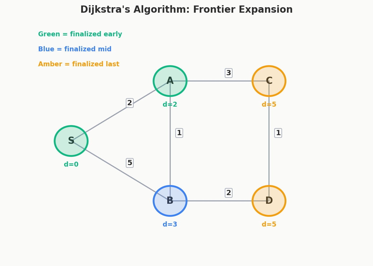
Dijkstra's algorithm maintains a set of finalized nodes whose shortest distances are known. At each step, it picks the unfinalized node \(u\) with the smallest tentative distance and declares that distance final.
This is a greedy choice: we commit to \(u\)'s distance without examining every possible path. Why is it safe?
The greedy choice property. Suppose \(u\) is the unfinalized node with the smallest tentative distance \(d[u]\). Any other path from \(s\) to \(u\) must pass through some other unfinalized node \(w\) first. But \(d[w] \geq d[u]\) (since \(u\) has the minimum), and the edge from \(w\) toward \(u\) adds a non-negative weight. So any alternative path has total length \(\geq d[w] \geq d[u]\).
Therefore \(d[u]\) is already optimal. Once finalized, it never improves.
This is exactly the structure from Lesson 1: an irrevocable local decision that is globally safe because no future choice can produce a better outcome.
The Algorithm
- Set \(d[s] = 0\) and \(d[v] = \infty\) for all other nodes.
- Insert \((0, s)\) into a min-heap.
- Extract the minimum \((d, u)\) from the heap.
- If \(u\) is already finalized, skip it.
- Mark \(u\) as finalized.
- For each neighbor \(v\) of \(u\) with edge weight \(w\): if \(d[u] + w < d[v]\), update \(d[v] = d[u] + w\) and push \((d[v], v)\) into the heap. This step is called relaxation.
- Repeat from step 3 until the heap is empty.
Full Trace
Consider a 6-node directed graph with source \(s = 1\):
Edges:
1 -> 2  (weight 7)
1 -> 3  (weight 9)
1 -> 6  (weight 14)
2 -> 3  (weight 10)
2 -> 4  (weight 15)
3 -> 4  (weight 11)
3 -> 6  (weight 2)
4 -> 5  (weight 6)
6 -> 5  (weight 9)
We trace the algorithm step by step. The distance array starts as \(d = [0, \infty, \infty, \infty, \infty, \infty]\) for nodes \(1\) through \(6\).
Step 1: Extract node 1 (distance 0)
| Neighbor | Edge Weight | Candidate | Old \(d\) | Update? | New \(d\) |
|---|---|---|---|---|---|
| 2 | 7 | \(0+7=7\) | \(\infty\) | Yes | 7 |
| 3 | 9 | \(0+9=9\) | \(\infty\) | Yes | 9 |
| 6 | 14 | \(0+14=14\) | \(\infty\) | Yes | 14 |
Distance array: \([0, 7, 9, \infty, \infty, 14]\). Heap: \(\{(7,2), (9,3), (14,6)\}\).
Step 2: Extract node 2 (distance 7)
| Neighbor | Edge Weight | Candidate | Old \(d\) | Update? | New \(d\) |
|---|---|---|---|---|---|
| 3 | 10 | \(7+10=17\) | 9 | No | 9 |
| 4 | 15 | \(7+15=22\) | \(\infty\) | Yes | 22 |
Distance array: \([0, 7, 9, 22, \infty, 14]\). Heap: \(\{(9,3), (14,6), (22,4)\}\).
Step 3: Extract node 3 (distance 9)
| Neighbor | Edge Weight | Candidate | Old \(d\) | Update? | New \(d\) |
|---|---|---|---|---|---|
| 4 | 11 | \(9+11=20\) | 22 | Yes | 20 |
| 6 | 2 | \(9+2=11\) | 14 | Yes | 11 |
Distance array: \([0, 7, 9, 20, \infty, 11]\). Heap: \(\{(11,6), (14,6), (20,4), (22,4)\}\).
Note: the heap now contains stale entries \((14, 6)\) and \((22, 4)\). These will be skipped when extracted because those nodes will already be finalized.
Step 4: Extract node 6 (distance 11)
| Neighbor | Edge Weight | Candidate | Old \(d\) | Update? | New \(d\) |
|---|---|---|---|---|---|
| 5 | 9 | \(11+9=20\) | \(\infty\) | Yes | 20 |
Distance array: \([0, 7, 9, 20, 20, 11]\). Heap: \(\{(14,6), (20,4), (20,5), (22,4)\}\).
Step 5: Extract (14, 6) --- node 6 already finalized, skip.
Step 6: Extract node 4 (distance 20)
| Neighbor | Edge Weight | Candidate | Old \(d\) | Update? | New \(d\) |
|---|---|---|---|---|---|
| 5 | 6 | \(20+6=26\) | 20 | No | 20 |
Distance array: \([0, 7, 9, 20, 20, 11]\). Heap: \(\{(20,5), (22,4)\}\).
Step 7: Extract node 5 (distance 20). No outgoing edges.
Step 8: Extract (22, 4) --- already finalized, skip. Heap empty.
Final distances: \(d = [0, 7, 9, 20, 20, 11]\). At every step, the greedy choice was correct.
Why Negative Edges Break Dijkstra
The greedy choice property relies on a critical assumption: edge weights are non-negative. When this assumption fails, Dijkstra gives wrong answers.
Counterexample. Consider 3 nodes:
Dijkstra starting from node 1:
- Extract node 1 (\(d = 0\)). Relax: \(d[2] = 1\), \(d[3] = 5\). Heap: \(\{(1,2), (5,3)\}\).
- Extract node 2 (\(d = 1\)). Finalized. No outgoing edges from 2.
- Extract node 3 (\(d = 5\)). Relax edge \(3 \to 2\): candidate \(= 5 + (-10) = -5 < 1\). But node 2 is already finalized!
Dijkstra reports \(d[2] = 1\), but the true shortest path is \(1 \to 3 \to 2\) with cost \(5 + (-10) = -5\).
The greedy assumption failed: when we finalized node 2 with distance 1, we assumed no future path could beat it. But the negative edge from node 3 created a cheaper route discovered too late.
Lesson: Dijkstra requires non-negative edge weights. For graphs with negative edges (but no negative cycles), use Bellman-Ford.
Complexity
With a binary heap (standard priority_queue):
- Each node is extracted from the heap at most once: \(O(V)\) extractions.
- Each extraction costs \(O(\log V)\) (heap pop).
- Each edge is examined at most once during relaxation, and each relaxation may push to the heap: \(O(E)\) pushes, each costing \(O(\log V)\).
Total: \(O((V + E) \log V)\).
For dense graphs (\(E \approx V^2\)), this becomes \(O(V^2 \log V)\). A Fibonacci heap improves this to \(O(V \log V + E)\), but in competitive programming the binary heap version is standard and fast enough.
The Code
#include <bits/stdc++.h>
using namespace std;

int main() {
    ios_base::sync_with_stdio(false);
    cin.tie(NULL);

    int numNodes, numEdges;
    cin >> numNodes >> numEdges;

    vector<vector<pair<int, long long>>> adjacencyList(numNodes + 1);
    for (int i = 0; i < numEdges; i++) {
        int fromNode, toNode;
        long long edgeWeight;
        cin >> fromNode >> toNode >> edgeWeight;
        adjacencyList[fromNode].push_back({toNode, edgeWeight});
    }

    const long long INF = 1e18;
    vector<long long> shortestDistance(numNodes + 1, INF);
    vector<bool> visitedNodes(numNodes + 1, false);
    shortestDistance[1] = 0;

    auto comparator = [](pair<long long, int>& left, pair<long long, int>& right) {
        return left.first > right.first;
    };
    priority_queue<pair<long long, int>, vector<pair<long long, int>>, decltype(comparator)> minHeap(comparator);
    minHeap.push({0, 1});

    while (!minHeap.empty()) {
        auto [currentDistance, currentNode] = minHeap.top();
        minHeap.pop();

        if (visitedNodes[currentNode]) continue;
        visitedNodes[currentNode] = true;

        for (auto& [neighborNode, edgeWeight] : adjacencyList[currentNode]) {
            long long candidateDistance = currentDistance + edgeWeight;
            if (candidateDistance < shortestDistance[neighborNode]) {
                shortestDistance[neighborNode] = candidateDistance;
                minHeap.push({candidateDistance, neighborNode});
            }
        }
    }

    for (int node = 1; node <= numNodes; node++) {
        cout << (shortestDistance[node] == INF ? -1 : shortestDistance[node]);
        if (node < numNodes) cout << " ";
    }
    cout << "\n";

    return 0;
}
Key details to notice:
- Lambda comparator. The
comparatorlambda reverses the default max-heap into a min-heap by comparing with>instead of<. - Lazy deletion. Instead of decreasing keys in the heap (which
priority_queuedoes not support), we push duplicate entries and skip nodes that are already finalized. This is the standard competitive programming approach. visitedNodesguard. Without this check, we would process stale heap entries and potentially do \(O(E)\) redundant relaxations.long longdistances. Edge weights can be up to \(10^9\) and paths can have up to \(10^5\) edges, so distances can exceed \(2^{31}\).
Connection to Later Material
In Chapter 8 Lesson 2 (Implicit State Space Search), we extend Dijkstra to graphs that are never explicitly built. Instead of nodes being integers \(1\) to \(V\), a "node" becomes an entire state --- for example, a bitmask of visited cities, or a tuple \((position, fuel, time)\). The adjacency list is replaced by a function that generates neighbors on the fly.
The core algorithm is identical: extract the minimum-distance state, relax its neighbors, push improvements to the heap. The greedy choice property still holds because all transition costs remain non-negative. What changes is the scale of the state space --- often exponential --- which makes the heap essential for pruning states you never need to visit. If you understood the trace above, you already understand the engine behind those applications.
Try It
The starter code has the Dijkstra framework with the relaxation loop body empty. Fill in the two lines: update shortestDistance[neighborNode] and push to the heap when candidateDistance is an improvement.
Test case 1:
Trace: \(1 \xrightarrow{3} 2 \xrightarrow{1} 3 \xrightarrow{2} 4 \xrightarrow{4} 5\). Distances: \([0, 3, 4, 6, 10]\).
Test case 2:
Node 2 is only reachable directly. Node 3 is closer even though it appears second.
Test case 3 (unreachable node):
Node 4 has no incoming edges. Its distance stays \(\infty\), printed as \(-1\).
Predict before running: In test case 1, which node gets finalized third? Trace the heap state after extracting nodes 1 and 2 to figure it out.
Problems
| Problem | Link | Difficulty |
|---|---|---|
| CSES Shortest Routes I | cses.fi/problemset/task/1671 | Easy |
| CSES Shortest Routes II | cses.fi/problemset/task/1672 | Easy |
| CF 20C — Dijkstra? | codeforces.com/contest/20/problem/C | 1900 |
| CSES Flight Discount | cses.fi/problemset/task/1195 | Medium |
| LC 743 — Network Delay Time | leetcode.com/problems/network-delay-time | Medium |