Path Queries and RMQ

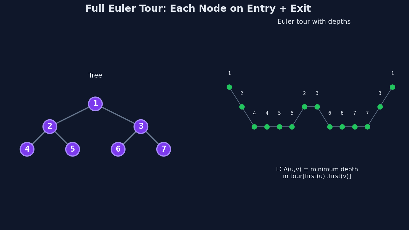
Full Euler tour records each node on entry and on return from every child

A Different Kind of Euler Tour

In the last two lessons, the DFS ordering recorded each node once — on entry. Now we need a different linearization: one that records a node every time the DFS visits it, including when it backtracks.

This is the Euler tour (sometimes called the "full Euler tour" to distinguish it from the DFS ordering). For a tree with \(n\) nodes, the Euler tour has exactly \(2n - 1\) entries.

Why do we need this? Because this tour encodes path information, not just subtree information. And path information is what we need to compute Lowest Common Ancestors.

Building the Euler Tour

The rule: every time the DFS is "at" a node — either entering it or returning to it after finishing a child — append that node to the tour.

For a tree rooted at node 1:

The DFS visits in this order:

Enter 1 → append 1
Enter 2 → append 2
Enter 4 → append 4
Backtrack to 2 → append 2
Enter 5 → append 5
Backtrack to 2 → append 2
Backtrack to 1 → append 1
Enter 3 → append 3
Backtrack to 1 → append 1

Euler tour: [1, 2, 4, 2, 5, 2, 1, 3, 1]

That's \(2 \times 5 - 1 = 9\) entries. Each node \(v\) appears exactly \((\text{degree}(v) + 1)\) times if we count the initial entry plus one return per child. But the total is always \(2n - 1\).

LCA from the Euler Tour

Record the depth of each node alongside the tour:

Index	0	1	2	3	4	5	6	7	8
Node	1	2	4	2	5	2	1	3	1
Depth	0	1	2	1	2	1	0	1	0

Also record the first occurrence of each node: the index where it first appears in the tour.

Node	First occurrence
1	0
2	1
3	7
4	2
5	4

The LCA Rule: \(LCA(u, v)\) is the node with the minimum depth in the Euler tour between the first occurrences of \(u\) and \(v\).

Example: LCA(4, 5).

First occurrence of 4 is index 2. First occurrence of 5 is index 4. Look at the segment \([2, 4]\):

Index	2	3	4
Node	4	2	5
Depth	2	1	2

Minimum depth is 1, at index 3, which is node 2. So \(LCA(4, 5) = 2\). Correct — 4 and 5 are both children of 2.

Example: LCA(4, 3).

First occurrence of 4 is index 2. First occurrence of 3 is index 7. Segment \([2, 7]\):

Index	2	3	4	5	6	7
Node	4	2	5	2	1	3
Depth	2	1	2	1	0	1

Minimum depth is 0, at index 6, which is node 1. So \(LCA(4, 3) = 1\). Correct — 4 is in the left subtree, 3 is in the right subtree, they meet at the root.

Why does this work? Between the first visit to \(u\) and the first visit to \(v\), the DFS must backtrack through their common ancestors. The highest it backtracks (shallowest depth) is exactly the LCA.

Sparse Table for O(1) RMQ

We need "minimum depth in a range" — a Range Minimum Query (RMQ). A sparse table gives us \(O(n \log n)\) preprocessing and \(O(1)\) per query.

The idea: precompute the answer for every range whose length is a power of 2. To answer a range \([l, r]\), overlap two precomputed ranges that together cover \([l, r]\).

Building the sparse table on our depth array:

Let \(st[i][k]\) = index of minimum depth in \([i, i + 2^k - 1]\).

Base case (\(k = 0\)): \(st[i][0] = i\) for all \(i\).

\(k = 1\) (ranges of length 2):

\(i\)	Range	Depths	Min index
0	[0,1]	0, 1	0
1	[1,2]	1, 2	1
2	[2,3]	2, 1	3
3	[3,4]	1, 2	3
4	[4,5]	2, 1	5
5	[5,6]	1, 0	6
6	[6,7]	0, 1	6
7	[7,8]	1, 0	8

\(k = 2\) (ranges of length 4):

\(i\)	Range	Min index
0	[0,3]	0
1	[1,4]	1
2	[2,5]	3
3	[3,6]	6
4	[4,7]	6
5	[5,8]	6

Answering a query: \(RMQ(2, 7)\). Length = 6. \(k = \lfloor \log_2 6 \rfloor = 2\). Check \(st[2][2]\) (range \([2,5]\), min index = 3, depth 1) and \(st[7 - 4 + 1][2] = st[4][2]\) (range \([4,7]\), min index = 6, depth 0). The overall minimum is at index 6, depth 0, node 1.

Two lookups. \(O(1)\).

The Code

vector<int> adjacency[200005];
int depth[200005];
int eulerTour[400005];
int eulerDepth[400005];
int firstOccurrence[200005];
int tourSize = 0;
int sparseTable[400005][20];
int logTable[400005];

void dfs(int node, int parent, int currentDepth) {
    depth[node] = currentDepth;
    firstOccurrence[node] = tourSize;
    eulerTour[tourSize] = node;
    eulerDepth[tourSize] = currentDepth;
    tourSize++;
    for (int child : adjacency[node]) {
        if (child != parent) {
            dfs(child, node, currentDepth + 1);
            eulerTour[tourSize] = node;
            eulerDepth[tourSize] = currentDepth;
            tourSize++;
        }
    }
}

void buildSparseTable() {
    logTable[1] = 0;
    for (int i = 2; i <= tourSize; i++)
        logTable[i] = logTable[i / 2] + 1;
    for (int i = 0; i < tourSize; i++)
        sparseTable[i][0] = i;
    for (int power = 1; (1 << power) <= tourSize; power++) {
        for (int i = 0; i + (1 << power) - 1 < tourSize; i++) {
            int left = sparseTable[i][power - 1];
            int right = sparseTable[i + (1 << (power - 1))][power - 1];
            sparseTable[i][power] = (eulerDepth[left] <= eulerDepth[right]) ? left : right;
        }
    }
}

int queryRMQ(int left, int right) {
    int length = right - left + 1;
    int k = logTable[length];
    int candidateLeft = sparseTable[left][k];
    int candidateRight = sparseTable[right - (1 << k) + 1][k];
    return (eulerDepth[candidateLeft] <= eulerDepth[candidateRight]) ? candidateLeft : candidateRight;
}

int lca(int u, int v) {
    int left = firstOccurrence[u];
    int right = firstOccurrence[v];
    if (left > right) swap(left, right);
    return eulerTour[queryRMQ(left, right)];
}

Complexity: \(O(n \log n)\) preprocessing, \(O(1)\) per LCA query.

When to Use This

This is the fastest LCA method for batch queries — when you know all queries upfront or simply need each one answered in \(O(1)\). The \(O(n \log n)\) preprocessing is a one-time cost.

In Chapter 12, we'll compare this with binary lifting (which is \(O(\log n)\) per query but also solves \(k\)-th ancestor). For now, remember: Euler tour + sparse table = \(O(1)\) LCA.

Try It

Predict before running: For the 5-node tree above, what is \(LCA(5, 3)\)? First occurrence of 5 is index 4, of 3 is index 7. Segment \([4, 7]\): depths are \([2, 1, 0, 1]\). Minimum is 0 at index 6, node 1.

Challenge: What happens if you query \(LCA(v, v)\)? The range is \([first[v], first[v]]\), a single element. The minimum is \(v\) itself. Correct — every node is its own LCA.

Challenge 2: The sparse table uses \(O(n \log n)\) memory. For \(n = 2 \times 10^5\), that's about \(4 \times 10^5 \times 18 \approx 7 \times 10^6\) integers. Around 28 MB. Tight but fine for most judges (256 MB limit).

Edge Cases to Watch For

first[u] > first[v] — query range is inverted: The RMQ expects first[u] <= first[v]. If not, swap them. Forgetting this swap returns a garbage minimum from an invalid range.
Sparse table column count too small: If \(2^{\text{MAXLOG}} <\) tour length, the table can't cover the full range. Always set the column count to \(\lceil \log_2(\text{tour length}) \rceil + 1\).

Problems

Problem	Link	Difficulty
CSES — Company Queries II	cses.fi/problemset/task/1688	Medium
CSES — Distance Queries	cses.fi/problemset/task/1135	Medium
CF 519E — A and B and Lecture Rooms	codeforces.com/problemset/problem/519/E	Hard