Non-Linear Wait
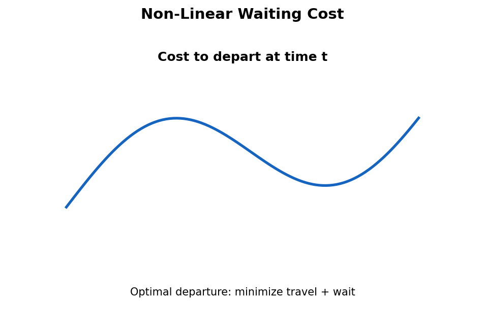
Rush hour traffic at 5 PM: crawling, miserable, 90 minutes to go 20 miles. Leave at 7 PM instead: 25 minutes, same route. Sometimes the fastest path isn't the one where you leave immediately. Sometimes you sit at a coffee shop and wait for the road to clear.
Lesson 1's trains had a clean FIFO property --- leaving earlier always meant arriving earlier. This lesson breaks that assumption. And Dijkstra still works, but only if you're clever about it.
The Setup: AtCoder abc204_e (Rush Hour 2)
\(N\) cities, \(M\) bidirectional roads. Road \(i\) connects \(A_i\) and \(B_i\). If you depart at time \(t\), the travel time is:
\(C_i\) is the base travel time. The \(D_i / (t+1)\) term is congestion that decreases as you depart later. Find the earliest arrival at city \(N\) starting from city 1 at time 0.
The Problem With Greedy Departure
In Lesson 1, we always departed as soon as possible. That was safe because FIFO held. Here, FIFO is violated:
| Depart time \(t\) | Travel cost (\(C=5, D=100\)) | Arrive |
|---|---|---|
| 0 | 5 + 100/1 = 105 | 105 |
| 4 | 5 + 100/5 = 25 | 29 |
| 9 | 5 + 100/10 = 15 | 24 |
| 99 | 5 + 100/100 = 6 | 105 |
Departing at \(t = 0\) gives arrival 105. Departing at \(t = 9\) gives arrival 24. Leaving later is massively better. But waiting too long (\(t = 99\)) is bad again --- the congestion savings don't offset the late start.
Key insight. The arrival time \(f(t) = t + C + \lfloor D/(t+1) \rfloor\) is convex-ish. It has a minimum, and we need to find it.
Finding the Optimal Departure
We want to minimize:
Treating this as continuous and differentiating:
So the optimal departure time is around \(\sqrt{D} - 1\). But we have two complications:
- Integer arithmetic. We need \(\lfloor D/(t+1) \rfloor\), not exact division.
- Arrival constraint. We can't depart before we arrive: \(t \geq \text{arrival\_time}\).
For the integer issue, check a few candidates near the continuous optimum:
For the arrival constraint, clamp:
The Full Calculation
auto best_arrival = [](long long arr, long long C, long long D)
    -> long long
{
    long long best = LLONG_MAX;
    long long t0 = max(arr, (long long)(sqrt((double)D) - 1));
    for (long long t = max(0LL, t0 - 1); t <= t0 + 2; t++) {
        if (t < arr) continue;
        long long cost = t + C + D / (t + 1);
        best = min(best, cost);
    }
    return best;
};
We try 3--4 candidates and take the minimum. This is \(O(1)\) per edge.
Gotcha. Don't forget
t0 - 1in the loop. Due to floor division, the integer optimum can be one less than the continuous optimum. Missing this gives WA on edge cases.
Why Dijkstra Still Works
FIFO is broken. If you arrive at \(u\) at time 3, the optimal departure might be time 9. A later arrival at \(u\) (say time 8) might use a different optimal departure (say time 9 again) and get the same result.
But Dijkstra still works because we compute the best possible arrival at \(v\) given our arrival at \(u\). The key property we need:
If \(t_1 \leq t_2\) (two arrivals at \(u\)), then \(\text{best\_arrival}(t_1) \leq \text{best\_arrival}(t_2)\).
Why? Arrival \(t_1\) can use all departure times \(\geq t_1\). Arrival \(t_2\) can only use departure times \(\geq t_2\). Since \(t_1 \leq t_2\), the set of options for \(t_1\) is a superset. A superset can't have a worse minimum.
Key insight. Even without FIFO on raw departure times, the optimized arrival function is monotone. Dijkstra needs monotonicity of the optimized cost, not of every individual departure.
Trace: 3-City Example
Cities: 1, 2, 3. Source = 1, Target = 3.
| Road | Cities | C | D |
|---|---|---|---|
| 1 | 1 -- 2 | 2 | 36 |
| 2 | 2 -- 3 | 1 | 16 |
| 3 | 1 -- 3 | 5 | 100 |
Road 1 (1->2): optimal \(t = \sqrt{36} - 1 = 5\). Arrive at \(t=0\), so we can wait.
| Depart \(t\) | Arrive at 2 |
|---|---|
| 0 | 0 + 2 + 36/1 = 38 |
| 4 | 4 + 2 + 36/5 = 13 |
| 5 | 5 + 2 + 36/6 = 13 |
| 6 | 6 + 2 + 36/7 = 13 |
Best via road 1: depart at 5, arrive at 13.
Road 3 (1->3) directly: optimal \(t = \sqrt{100} - 1 = 9\).
| Depart \(t\) | Arrive at 3 |
|---|---|
| 0 | 0 + 5 + 100 = 105 |
| 9 | 9 + 5 + 10 = 24 |
Best via road 3: depart at 9, arrive at 24.
Road 2 (2->3) from arrival time 13: optimal \(t = \sqrt{16} - 1 = 3\), but clamped to 13.
| Depart \(t\) | Arrive at 3 |
|---|---|
| 13 | 13 + 1 + 16/14 = 15 |
Dijkstra trace:
| Step | Pop (time, city) | Edge | Best arrive | Update? |
|---|---|---|---|---|
| 1 | (0, 1) | 1->2 | 13 | dist[2] = 13 |
| 1 | (0, 1) | 1->3 | 24 | dist[3] = 24 |
| 2 | (13, 2) | 2->3 | 15 | dist[3] = 15 |
| 3 | (15, 3) | target | --- | done |
Answer: 15.
Path: wait at city 1 until \(t=5\), ride to city 2 (arrive \(t=13\)), immediately depart to city 3 (arrive \(t=15\)). The direct route takes 24. Waiting saved 9 time units.
The "Wait Then Go" Pattern
This problem introduces a pattern you'll see repeatedly:
- You arrive at node \(u\) at time \(t\).
- The edge cost is a function of departure time: \(g(\text{depart})\).
- You're free to wait: \(\text{depart} \geq t\).
- Minimize \(\text{depart} + g(\text{depart})\) subject to \(\text{depart} \geq t\).
The solution is always the same:
- Find the unconstrained optimum \(t^*\).
- Clamp: \(\text{depart} = \max(t, t^*)\).
- Check a few integer neighbors for floor/ceiling effects.
Different problems give different \(g\) functions. This problem has \(g(t) = C + D/(t+1)\). Others might have piecewise-linear or step functions. The framework stays the same.
Edge Case: D = 0
When \(D = 0\), the edge cost is just \(C\) regardless of time. \(\sqrt{0} - 1 = -1\), which gets clamped to the arrival time. The formula degenerates cleanly to standard Dijkstra.
Gotcha. Make sure your
sqrtdoesn't produce negative candidates. Usemax(0LL, t0 - 1)as the loop start to avoid testing negative departure times.
Complexity
Same as Lesson 1: \(O((N + M) \log N)\). The optimal departure calculation is \(O(1)\) per edge --- just a square root and 3--4 comparisons. No state expansion needed.
Exercises
-
Manual optimization. Edge with \(C = 3, D = 48\). You arrive at time 2. What's the optimal departure? What's the arrival time?
-
Constraint interaction. You arrive at time 20. The unconstrained optimum is \(t = 7\). What departure do you use? Why is this still correct?
-
D very large. \(D = 10^{18}\). What's the approximate optimal departure time? Is there any overflow risk in
t + C + D/(t+1)?
Problems
| Problem | Link | Difficulty |
|---|---|---|
| AtCoder abc204_e --- Rush Hour 2 | atcoder.jp/contests/abc204/tasks/abc204_e | Hard |
| LC 1928 --- Minimum Cost to Reach Destination in Time | leetcode.com/problems/minimum-cost-to-reach-destination-in-time | Hard |