The Contribution Technique
The Problem
Here's a clean problem statement: given an array of integers, compute the sum of the minimum values of every contiguous subarray.
For example, A = [3, 1, 2, 4]. The subarrays and their minimums:
| Subarray | Min |
|---|---|
| [3] | 3 |
| [3,1] | 1 |
| [3,1,2] | 1 |
| [3,1,2,4] | 1 |
| [1] | 1 |
| [1,2] | 1 |
| [1,2,4] | 1 |
| [2] | 2 |
| [2,4] | 2 |
| [4] | 4 |
Sum = 3 + 1 + 1 + 1 + 1 + 1 + 1 + 2 + 2 + 4 = 17.
This is LeetCode 907 (Sum of Subarray Minimums). The brute force — enumerate all O(N^2) subarrays and find each minimum — is too slow for N up to 10^5.
The Flip
The brute force asks: "For each subarray, what's its minimum?" That's an O(N^2) question because there are O(N^2) subarrays.
The contribution technique flips the question: "For each element, how many subarrays is it the minimum of?"
If we know that A[i] is the minimum of exactly C[i] subarrays, then its total contribution to the answer is A[i] * C[i]. Sum all contributions and you're done.
This flip turns an O(N^2) problem into O(N), because computing C[i] for every element just requires the left and right boundaries — which the monotonic stack gives us in O(N).
Counting Subarrays
Say A[i]'s left boundary is L and right boundary is R. We know A[i] is the minimum of the subarray A[L+1 .. R-1]. But it's also the minimum of every subarray within that range that includes index i.
How many such subarrays are there? A subarray that includes i needs:
- A start point anywhere from
L+1toi. That's(i - L)choices. - An end point anywhere from
itoR-1. That's(R - i)choices.
Every combination of start and end gives a distinct subarray, and A[i] is the minimum of all of them. So:
Total contribution of A[i]:
That's it. Three lines of insight, and the whole problem collapses.
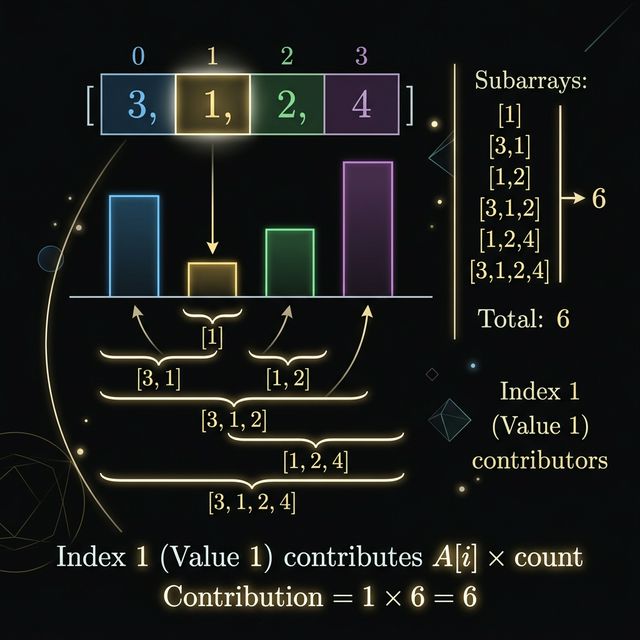
Walkthrough: [3, 1, 2, 4]
Let's compute boundaries. We need the nearest strictly smaller element on each side.
i |
A[i] |
L[i] |
R[i] |
Left choices (i-L) |
Right choices (R-i) |
Count | Contribution |
|---|---|---|---|---|---|---|---|
| 0 | 3 | 1 (*) | 1 | 0 - (-1) = 1 (*) | 1 - 0 = 1 | 1 | 3 |
| 1 | 1 | -1 | 4 | 1 - (-1) = 2 | 4 - 1 = 3 | 6 | 6 |
| 2 | 2 | 1 | 4 | 2 - 1 = 1 | 4 - 2 = 2 | 2 | 4 |
| 3 | 4 | 2 | 4 | 3 - 2 = 1 | 4 - 3 = 1 | 1 | 4 |
Wait — let me redo index 0 carefully. A[0] = 3. Looking left: nothing there, so L[0] = -1. Looking right: A[1] = 1 < 3, so R[0] = 1. Left choices = 0 - (-1) = 1. Right choices = 1 - 0 = 1. Count = 1. Contribution = 3 * 1 = 3.
Totals: 3 + 6 + 4 + 4 = 17. Matches our brute force.
Let's verify element 1 (value 1). It's the min of 6 subarrays. Which ones? Start at index 0 or 1 (2 choices), end at index 1, 2, or 3 (3 choices). That gives subarrays [3,1], [3,1,2], [3,1,2,4], [1], [1,2], [1,2,4]. All have min 1. Six subarrays, contribution 1 * 6 = 6. Perfect.
The Duplicate Problem
There's a trap. What happens when the array has equal elements?
Take A = [1, 1]. The subarrays are [1], [1,1], [1]. The sum of minimums is 1 + 1 + 1 = 3.
If we use strictly smaller (<) for both boundaries:
- Index 0: L=−1, R=2. Count = (0−(−1)) * (2−0) = 1 * 2 = 2. Contribution = 2.
- Index 1: L=−1, R=2. Count = (1−(−1)) * (2−1) = 2 * 1 = 2. Contribution = 2.
- Total = 4. Wrong. We overcounted.
The problem: the subarray [1,1] got counted twice — once for index 0 (it's in its range) and once for index 1 (also in its range). When two elements have the same value, their ranges of dominance overlap, and shared subarrays get double-counted.
The fix: break ties asymmetrically. Use strict inequality on one side and non-strict on the other. Specifically:
- Left boundary: pop while
A[stack.top()] >= A[i](strict less on boundary — look for strictly smaller). - Right boundary: pop while
A[stack.top()] > A[i](non-strict on boundary — look for smaller or equal).
This means: when two elements are equal, the leftmost one "owns" the range. The rightmost one's boundary gets cut short by the equal element to its left.
Let's redo [1, 1] with the asymmetric rule:
- Index 0: L=−1 (strict), R=1 (right boundary uses >, and A[1]=1 is not > A[0]=1, so... wait, let me be precise). Right scan for index 0: look for the nearest
j > 0whereA[j] <= A[0]. That's index 1. SoR[0] = 1. Count = 1 * 1 = 1. Contribution = 1. - Index 1: L=−1 (left scan: look for
A[j] < A[1], nothing qualifies). Wait, that doesn't seem right either.
Let me state it precisely. The convention is:
- Left boundary: nearest index
j < iwithA[j] < A[i](strictly smaller). Pop condition:A[top] >= A[i]. - Right boundary: nearest index
j > iwithA[j] <= A[i](smaller or equal). Pop condition:A[top] > A[i].
For [1, 1]:
- Index 0: L=−1. For right: scan right, looking for
A[j] <= 1. Index 1 has value 1, and 1 <= 1, soR[0] = 1. Count = 1 * 1 = 1. Contribution = 1. - Index 1: L=−1 (no element strictly less than 1 to the left). R=2 (nothing <= 1 to the right). Count = 2 * 1 = 2. Contribution = 2.
- Total = 3. Correct!
The subarray [1,1] is now owned by index 1 only (it's in index 1's range but not in index 0's range because R[0] = 1 cuts it off). No double-counting.
This asymmetric boundary trick is the single most common mistake people make with the contribution technique. Always use strict on one side and non-strict on the other when the array can have duplicates.
The General Formula
For Sum of Subarray Minimums:
Where L[i] uses < (nearest strictly smaller to the left) and R[i] uses <= (nearest smaller-or-equal to the right).
For Sum of Subarray Maximums, flip everything:
L[i]= nearest strictly greater to the leftR[i]= nearest greater-or-equal to the right- Same formula:
A[i] * (i - L[i]) * (R[i] - i)
And if the problem asks for "Sum of Subarray Ranges" (the difference between max and min for each subarray), you compute both sums separately and subtract.
Don't Forget the Modular Arithmetic
These problems almost always ask for the answer modulo 10^9 + 7. A few things to watch:
- The product
A[i] * (i - L) * (R - i)can overflow evenlong longif you're not careful. Multiply in stages and take mod at each step. (i - L)and(R - i)are always positive, so no negative mod issues here.- But if you ever compute a difference of two modular sums, you might get a negative result. Add MOD before taking mod:
((a - b) % MOD + MOD) % MOD.
The Bigger Picture
The contribution technique isn't limited to sum-of-minimums. The core idea — "instead of iterating over all subarrays and computing a property, iterate over all elements and count how many subarrays each element contributes to" — shows up in many forms:
- Sum of subarray minimums / maximums (what we just covered)
- Sum of subarray ranges (max - min for each subarray)
- Counting subarrays where a given element is the min/max
- Weighted contribution problems where each element's contribution depends on its range
Every one of these follows the same skeleton: compute boundaries with the monotonic stack, multiply out the contribution, sum up. Once you internalize this pattern, these problems all feel like the same problem wearing different costumes.