When Dijkstra Breaks
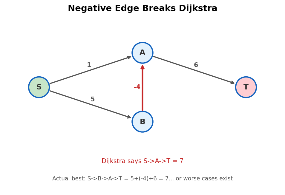
Dijkstra is not a universal shortest-path algorithm. Hand it a graph with a single negative edge and it can return the wrong answer — silently, confidently, with no error or warning. Understanding exactly why it breaks is more important than memorizing the fix, because the failure reveals the hidden assumption behind every greedy algorithm.
A Concrete Counterexample
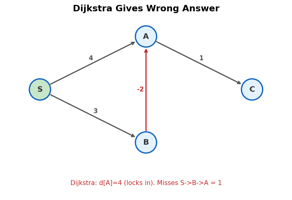
Four nodes, four edges:
Edges: 0→1 (5), 0→2 (2), 2→3 (1), 1→3 (-4).
The true shortest path from 0 to 3 is 0→1→3 with cost \(5 + (-4) = 1\).
Dijkstra's Trace
| Step | Pop (d, u) | dist[] | PQ | Note |
|---|---|---|---|---|
| Init | — | [0, ∞, ∞, ∞] | {(0,0)} | |
| 1 | (0, 0) | [0, 5, 2, ∞] | {(2,2), (5,1)} | Relax 0→1 and 0→2. |
| 2 | (2, 2) | [0, 5, 2, 3] | {(3,3), (5,1)} | Relax 2→3: 2+1=3. |
| 3 | (3, 3) | [0, 5, 2, 3] | {(5,1)} | Node 3 popped and finalized at 3. |
| 4 | (5, 1) | [0, 5, 2, 1] | {} | Relax 1→3: 5+(-4)=1 < 3. But 3 is already finalized! |
With the standard if (d > dist[u]) continue check, step 3 finalizes node 3 at distance 3. Step 4 pushes a better distance for node 3 into the PQ, but when that entry is popped, node 3 is already processed. Dijkstra reports dist[3] = 3. The correct answer is 1.
Gotcha. Some lazy-deletion implementations will process the updated entry and accidentally get the right answer. Don't be fooled — correctness by luck is not correctness. If your graph can have negative edges, Dijkstra's proof of correctness does not apply.
Why the Greedy Argument Breaks
Recall the proof from Lesson 1: when we pop node \(u\) from the PQ, its distance is optimal because any alternative path through an unfinished node \(x\) must have length \(\geq\) dist[x] \(\geq\) dist[u], and adding more non-negative edges can only make it longer.
With negative edges, "adding more edges can only make it longer" is false. A path through \(x\) can pick up a negative edge and end up shorter than dist[u]. The node we finalized early might not actually be optimal.
The proof breaks at one specific line: we assumed that extending a path with more edges increases its cost. Negative edges violate this assumption. A longer path (more edges) can have a shorter total weight.
Key insight. Dijkstra is greedy. Greedy works when local optimality implies global optimality. Negative edges break this because a locally suboptimal choice (longer path now) can become globally optimal (shorter path after a negative edge).
A Simpler Way to See It
Think of Dijkstra as making a permanent commitment. When it pops a node, it says: "I'm done with you. Your distance is final." With non-negative edges, this commitment is safe — no future discovery can improve a finalized node.
With negative edges, Dijkstra makes premature commitments. It finalizes node 3 at distance 3 before discovering the cheaper route through node 1. By the time it processes node 1, the damage is done.
Negative Cycles: Shortest Path is Undefined
A negative cycle is a cycle whose total edge weight is negative. If such a cycle is reachable from the source and can reach the destination, the shortest path is \(-\infty\) — you can loop around the cycle forever, decreasing the distance each time.
Path 0→1→2→1→2→1→2→...→target costs \(1 + k \times (-1)\) for \(k\) loops. As \(k \to \infty\), cost approaches \(-\infty\).
Neither Dijkstra nor standard Bellman-Ford can find a finite shortest path here. But Bellman-Ford can detect the cycle — Dijkstra cannot even do that.
The Decision Flowchart
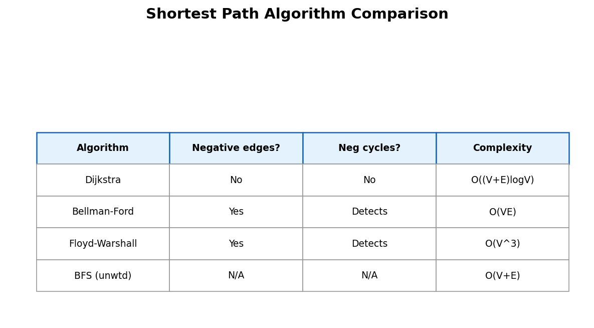
Before writing shortest-path code, answer two questions: (1) can weights be negative? (2) do you need single-source or all-pairs?
| Condition | Algorithm | Time |
|---|---|---|
| All weights \(\geq 0\) | Dijkstra | \(O((V+E) \log V)\) |
| Negative weights, no negative cycles | Bellman-Ford | \(O(VE)\) |
| Need to detect negative cycles | Bellman-Ford (Nth iteration) | \(O(VE)\) |
| All-pairs, \(V \leq 500\) | Floyd-Warshall | \(O(V^3)\) |
| Unweighted | BFS | \(O(V+E)\) |
| Weights 0 or 1 only | 0-1 BFS (deque) | \(O(V+E)\) |
Key insight. The algorithm choice is determined by the problem constraints, not by personal preference. Check edge weight signs and query type first.
Side-by-Side: Dijkstra vs Bellman-Ford
Here's both algorithms on the 4-node counterexample:
#include <bits/stdc++.h>
using namespace std;

int main() {
    int n = 4;
    struct Edge { int u, v; long long w; };
    vector<Edge> edges = {{0,1,5}, {0,2,2}, {2,3,1}, {1,3,-4}};

    // Build adjacency list for Dijkstra
    vector<vector<pair<int,long long>>> adj(n);
    for (auto [u, v, w] : edges)
        adj[u].push_back({v, w});

    // --- Dijkstra ---
    vector<long long> dd(n, LLONG_MAX);
    dd[0] = 0;
    priority_queue<pair<long long,int>,
                   vector<pair<long long,int>>, greater<>> pq;
    pq.push({0, 0});
    vector<bool> finalized(n, false);
    while (!pq.empty()) {
        auto [d, u] = pq.top(); pq.pop();
        if (finalized[u]) continue;
        finalized[u] = true;
        for (auto [v, w] : adj[u]) {
            if (dd[u] + w < dd[v]) {
                dd[v] = dd[u] + w;
                pq.push({dd[v], v});
            }
        }
    }
    cout << "Dijkstra dist[3] = " << dd[3] << "\n";
    // Prints 3 (WRONG — true answer is 1)

    // --- Bellman-Ford ---
    vector<long long> bf(n, LLONG_MAX);
    bf[0] = 0;
    for (int i = 0; i < n - 1; i++)
        for (auto [u, v, w] : edges)
            if (bf[u] != LLONG_MAX && bf[u] + w < bf[v])
                bf[v] = bf[u] + w;
    cout << "Bellman-Ford dist[3] = " << bf[3] << "\n";
    // Prints 1 (CORRECT)
}
Dijkstra gives 3. Bellman-Ford gives 1. The difference is that Bellman-Ford doesn't finalize nodes — it relaxes all edges repeatedly until convergence.
Preview: The Potential Function Trick
Some problems look like they have negative edges but can be transformed to avoid them. Johnson's algorithm assigns a potential \(h(v)\) to each node and reweights edge \((u, v, w)\) as \(w' = w + h(u) - h(v)\). If potentials come from one Bellman-Ford run, all reweighted edges become non-negative, and Dijkstra works again.
This is an advanced technique we'll revisit later. The takeaway for now: negative edges don't always force \(O(VE)\) Bellman-Ford. Sometimes you can transform the problem back into Dijkstra territory.
Common Mistakes
Mistake 1: "I'll just use Bellman-Ford everywhere"
Bellman-Ford is \(O(VE)\). For \(V = 10^5\) and \(E = 2 \times 10^5\), that's \(2 \times 10^{10}\) operations. Far too slow. Use Dijkstra when weights are non-negative.
Mistake 2: "Negative edges means negative cycles"
No. A graph can have negative edges without any negative cycle. Example: a DAG with negative weights. Bellman-Ford handles these correctly — shortest paths are finite and well-defined.
Mistake 3: "Just check if the answer changes"
Some people try to detect Dijkstra failures by running it twice. This doesn't work reliably. If the graph has negative edges, switch algorithms — don't try to patch Dijkstra.
Exercises
-
Construct a failure. Create a 3-node directed graph with one negative edge where Dijkstra (with finalized-node tracking) reports the wrong answer.
-
Can BFS handle negatives? If all edge weights are either \(+1\) or \(-1\), does BFS find shortest paths? Why or why not?
-
Count the cost. For \(V = 2500\), \(E = 5000\): Dijkstra does approximately \(7000 \times \log(5000) \approx 85{,}000\) operations. Bellman-Ford does \(2500 \times 5000 = 12{,}500{,}000\). That's a ~150x slowdown. When is this acceptable?
Problems
| Problem | Link | Difficulty |
|---|---|---|
| CSES — High Score | cses.fi/problemset/task/1673 | Medium |
| LC 787 — Cheapest Flights Within K Stops | leetcode.com/problems/cheapest-flights-within-k-stops | Medium |
| CSES — Cycle Finding | cses.fi/problemset/task/1197 | Medium |
| LC 743 — Network Delay Time | leetcode.com/problems/network-delay-time | Medium |