Antimatroids and Scheduling
The Other Side of the Greedoid Coin
Matroids capture "downward closure" — every subset of a feasible set is feasible. This gives Kruskal, graphic matroids, and the theory behind why greedy on minimum spanning trees works. But there is a dual structure, equally powerful, that captures the opposite idea.
An antimatroid is a greedoid \((\mathcal{E}, \mathcal{F})\) satisfying the upward closure (or accessibility) property:
In plain English: gaining more resources never restricts your options. If you can add element \(x\) when you have a small feasible set \(A\), you can also add \(x\) when you have a larger feasible set \(B\) that contains \(A\).
This is the exact opposite of a matroid's downward closure. In a matroid, having fewer elements keeps you feasible. In an antimatroid, having more elements keeps you flexible. Where matroids say "subsets of good sets are good," antimatroids say "if a move is legal in a restricted state, it stays legal in any richer state."
The Greedy Choice: When a problem has antimatroid structure, reverse greedy works — build the solution from the end, picking the "best" available element at each step, peeling from the top rather than building from the bottom.
Four Families of Antimatroids
Antimatroids arise naturally in combinatorics, geometry, and graph theory. Here are the four most important families.
Poset Antimatroid
Given a DAG (representing precedence constraints), the feasible sets are the downward-closed subsets: a set \(S\) is feasible if every predecessor of every element in \(S\) is also in \(S\).
The upward closure property holds because if you can add an element \(x\) (all its predecessors are present) in a smaller set \(A\), those predecessors are also present in any larger set \(B \supseteq A\).
Application: Machine scheduling with precedence constraints. This is where Lawler's 1973 algorithm lives, and it is the centerpiece of this lesson.
Shelling Antimatroid
Start with a set of points. The feasible sets are those obtainable by repeatedly removing vertices of the convex hull. At each step, any vertex currently on the convex hull can be removed — having more remaining points never prevents a hull vertex from being removable.
A deep theorem states that every antimatroid is isomorphic to a shelling antimatroid in a sufficiently high-dimensional space. This makes shelling antimatroids the "universal" model, just as vector matroids are representable over large enough fields.
Point Search (BFS) Antimatroid
Fix a root vertex \(r\) in a connected graph. The feasible sets are those reachable from \(r\) by BFS — sets \(S\) such that \(r \in S\) and every vertex in \(S\) has a neighbor that was added to \(S\) before it.
Upward closure holds because having more explored vertices only gives BFS more frontier edges to explore. This explains at a structural level why BFS is greedy-optimal for shortest paths in unweighted graphs: the set of reachable vertices forms an antimatroid, and BFS is the natural greedy algorithm on it.
Chip-Firing Antimatroid
Place chips on vertices of a directed graph. A vertex can "fire" if it has at least as many chips as out-edges. Firing sends one chip along each out-edge. The key property: the order of firings doesn't matter — if multiple vertices can fire, the final configuration is the same regardless of firing order. This confluence gives an antimatroid structure. Chip-firing is an active research topic connecting combinatorics, algebraic geometry, and tropical mathematics.
Lawler's Machine Scheduling Algorithm (1973)
This is the classical algorithm that demonstrates antimatroid structure in action. The problem is deceptively simple.
Problem: You have \(n\) jobs. Job \(j\) has processing time \(p_j\) and deadline \(d_j\). There are precedence constraints: some jobs must finish before others can start. You run one job at a time on a single machine, starting at time 0. Minimize the maximum lateness \(\max_j (C_j - d_j)\), where \(C_j\) is the completion time of job \(j\).
Without precedence constraints, this is easy: sort by deadline (Earliest Deadline First). But precedence constraints break the sorted order — you might need to run a prerequisite with a late deadline before a dependent job with an early deadline.
The Reverse-Greedy Insight
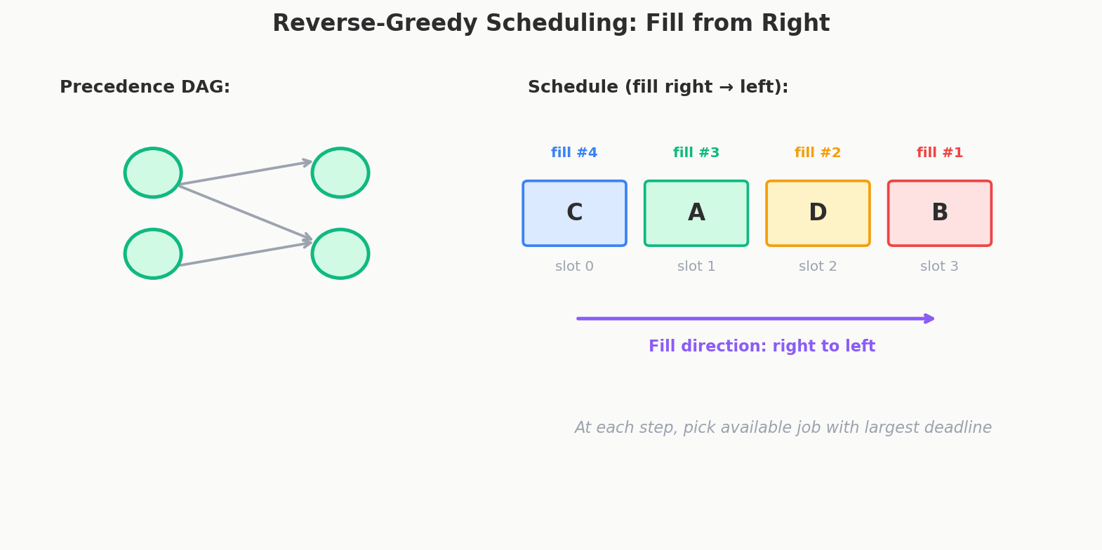
Lawler's observation: build the schedule backwards. At each step, look at which jobs have no unscheduled successors (jobs that could go last among the remaining unscheduled jobs without violating any precedence constraint). Among these available jobs, pick the one with the largest deadline.
Why largest deadline last? A job placed at the end of the schedule has the latest completion time. By putting the job with the largest deadline there, we minimize the worst-case lateness at that position. The antimatroid structure guarantees that "peeling off" the best available job from the end produces an optimal schedule.
Traced Example: 5 Jobs with Precedence
Consider 5 jobs with the following data:
| Job | \(p_j\) | \(d_j\) |
|---|---|---|
| 0 | 2 | 6 |
| 1 | 3 | 8 |
| 2 | 1 | 4 |
| 3 | 4 | 12 |
| 4 | 2 | 10 |
Precedence constraints (must finish before): \(0 \to 2\) (job 0 before job 2), \(1 \to 4\) (job 1 before job 4).
Total processing time: \(2 + 3 + 1 + 4 + 2 = 12\).
Step 1: Fill position 4 (last slot). Remaining: \(\{0, 1, 2, 3, 4\}\).
A job is available if no unscheduled job depends on it. Job 0 has successor 2 (unscheduled) — not available. Job 1 has successor 4 (unscheduled) — not available. Jobs 2, 3, 4 have no unscheduled successors — all available.
Among \(\{2, 3, 4\}\), largest deadline is job 3 (\(d_3 = 12\)). Place job 3 in position 4.
Step 2: Fill position 3. Remaining: \(\{0, 1, 2, 4\}\).
Job 0 has successor 2 (still unscheduled) — not available. Job 1 has successor 4 (still unscheduled) — not available. Jobs 2 and 4 — available.
Among \(\{2, 4\}\), largest deadline is job 4 (\(d_4 = 10\)). Place job 4 in position 3.
Step 3: Fill position 2. Remaining: \(\{0, 1, 2\}\).
Job 0 has successor 2 (unscheduled) — not available. Job 1 now has successor 4 (already scheduled) — available. Job 2 — available.
Among \(\{1, 2\}\), largest deadline is job 1 (\(d_1 = 8\)). Place job 1 in position 2.
Step 4: Fill position 1. Remaining: \(\{0, 2\}\).
Job 0 has successor 2 (unscheduled) — not available. Job 2 — available. Only choice: job 2 in position 1.
Step 5: Fill position 0. Only job 0 remains. Place job 0 in position 0.
Final schedule: \([0, 2, 1, 4, 3]\).
| Position | Job | \(p_j\) | Start | \(C_j\) | \(d_j\) | Lateness \(C_j - d_j\) |
|---|---|---|---|---|---|---|
| 0 | 0 | 2 | 0 | 2 | 6 | \(-4\) |
| 1 | 2 | 1 | 2 | 3 | 4 | \(-1\) |
| 2 | 1 | 3 | 3 | 6 | 8 | \(-2\) |
| 3 | 4 | 2 | 6 | 8 | 10 | \(-2\) |
| 4 | 3 | 4 | 8 | 12 | 12 | \(0\) |
Maximum lateness: \(0\). Every job finishes by its deadline.
Why the Antimatroid Structure Matters
The set of "schedulable suffixes" forms a poset antimatroid. The available jobs at each reverse step are exactly the elements that can extend the current feasible set. The upward closure property guarantees that once a job becomes available (all its successors are scheduled), it remains available as we schedule more jobs — our options never shrink as we progress. This is precisely what makes the greedy exchange argument work: if some other schedule were better, we could swap elements using the antimatroid exchange property and contradict optimality.
Convex Geometries: The Dual View
Every antimatroid has a dual called a convex geometry. Where antimatroids describe "what you can build," convex geometries describe "what is enclosed."
A convex geometry is a family \(\mathcal{C}\) of subsets (the "convex sets") that is closed under intersection and has the anti-exchange property. The key operation is the closure operator \(\tau\): for a set \(X\), \(\tau(X)\) is the smallest convex set containing \(X\).
The anti-exchange property states:
Think of actual convex hulls in the plane. If adding point \(y\) to a set \(X\) causes point \(z\) to fall inside the convex hull, then adding \(z\) to \(X\) will NOT cause \(y\) to fall inside. The relationship is asymmetric — \(y\) "covers" \(z\) but not the other way around.
The complements of a convex geometry's convex sets form an antimatroid. The closure operator dualizes to the antimatroid's feasible set system. This duality is not just theoretical — it provides an alternative proof technique for scheduling algorithms. Instead of reasoning about "what jobs can I add next" (antimatroid view), you can reason about "what jobs are forced by precedence constraints" (convex geometry view).
The Complete Hierarchy
Every algorithm you have encountered in this course fits somewhere in this classification:
GREEDOID
 |-- MATROID (downward-closed)
 |    |-- Graphic (Kruskal)
 |    |-- Vector (linear algebra)
 |    +-- Transversal (bipartite matching)
 |
 |-- ANTIMATROID (upward-closed)
 |    |-- Poset (scheduling / Lawler)
 |    |-- Shelling (convex hull peeling)
 |    |-- Point Search (BFS)
 |    +-- Chip-Firing (combinatorial games)
 |
 |-- INTERVAL GREEDOID (local union property)
 |    |-- Local Forest (Prim, Dijkstra)
 |    +-- Clique Elimination (chordal graphs)
 |
 +-- OTHER
      |-- Blossom (matching)
      |-- Gaussian Elimination
      +-- Ear Decomposition
The two main branches — matroids and antimatroids — are in a precise sense dual. Matroids select independent subsets greedily (build up from nothing). Antimatroids select feasible extensions greedily (often in reverse). Interval greedoids sit between them, requiring only a weaker "local" exchange property that suffices for algorithms like Prim and Dijkstra that grow from a single source.
Understanding where your problem sits in this hierarchy tells you which greedy strategy to try:
- Matroid structure \(\Rightarrow\) forward greedy (sort + pick the best compatible element)
- Antimatroid structure \(\Rightarrow\) reverse greedy (peel from the end, pick the element with most slack)
- Interval greedoid \(\Rightarrow\) local greedy (grow from a source, pick the best adjacent extension)
- No greedoid structure \(\Rightarrow\) greedy alone won't work; reach for DP, network flow, or undo tricks
The Code
An efficient implementation of Lawler's algorithm uses a topological sort framework. We track in-degree from the "reverse" perspective: an edge \(u \to v\) in the precedence DAG means \(u\) must come before \(v\), so in our reverse construction, \(v\) must be scheduled (placed) before \(u\).
#include <bits/stdc++.h>
using namespace std;

int main() {
    ios_base::sync_with_stdio(false);
    cin.tie(NULL);

    int numJobs;
    cin >> numJobs;

    vector<int> processingTime(numJobs);
    vector<int> deadline(numJobs);
    for (int job = 0; job < numJobs; job++) {
        cin >> processingTime[job] >> deadline[job];
    }

    int numEdges;
    cin >> numEdges;

    vector<vector<int>> successors(numJobs);
    vector<int> unscheduledSuccessorCount(numJobs, 0);
    for (int edge = 0; edge < numEdges; edge++) {
        int before, after;
        cin >> before >> after;
        successors[before].push_back(after);
        unscheduledSuccessorCount[before]++;
    }

    priority_queue<pair<int, int>> availableJobs;
    for (int job = 0; job < numJobs; job++) {
        if (unscheduledSuccessorCount[job] == 0) {
            availableJobs.push({deadline[job], job});
        }
    }

    vector<int> schedule(numJobs);

    for (int position = numJobs - 1; position >= 0; position--) {
        auto [bestDeadline, chosenJob] = availableJobs.top();
        availableJobs.pop();

        schedule[position] = chosenJob;

        for (int predecessor = 0; predecessor < numJobs; predecessor++) {
            for (int successor : successors[predecessor]) {
                if (successor == chosenJob) {
                    unscheduledSuccessorCount[predecessor]--;
                    if (unscheduledSuccessorCount[predecessor] == 0) {
                        availableJobs.push({deadline[predecessor], predecessor});
                    }
                }
            }
        }
    }

    int currentTime = 0;
    int maxLateness = INT_MIN;
    for (int position = 0; position < numJobs; position++) {
        int job = schedule[position];
        currentTime += processingTime[job];
        int lateness = currentTime - deadline[job];
        maxLateness = max(maxLateness, lateness);
    }

    cout << maxLateness << "\n";
    for (int position = 0; position < numJobs; position++) {
        cout << schedule[position] << " \n"[position == numJobs - 1];
    }

    return 0;
}
For better asymptotic performance, store reverse adjacency lists so that when job \(v\) is scheduled, you can directly decrement the successor count of each predecessor of \(v\):
#include <bits/stdc++.h>
using namespace std;

int main() {
    ios_base::sync_with_stdio(false);
    cin.tie(NULL);

    int numJobs;
    cin >> numJobs;

    vector<int> processingTime(numJobs);
    vector<int> deadline(numJobs);
    for (int job = 0; job < numJobs; job++) {
        cin >> processingTime[job] >> deadline[job];
    }

    int numEdges;
    cin >> numEdges;

    vector<vector<int>> reversePrecedence(numJobs);
    vector<int> unscheduledSuccessorCount(numJobs, 0);
    for (int edge = 0; edge < numEdges; edge++) {
        int before, after;
        cin >> before >> after;
        reversePrecedence[after].push_back(before);
        unscheduledSuccessorCount[before]++;
    }

    priority_queue<pair<int, int>> availableJobs;
    for (int job = 0; job < numJobs; job++) {
        if (unscheduledSuccessorCount[job] == 0) {
            availableJobs.push({deadline[job], job});
        }
    }

    vector<int> schedule(numJobs);

    for (int position = numJobs - 1; position >= 0; position--) {
        auto [bestDeadline, chosenJob] = availableJobs.top();
        availableJobs.pop();

        schedule[position] = chosenJob;

        for (int predecessor : reversePrecedence[chosenJob]) {
            unscheduledSuccessorCount[predecessor]--;
            if (unscheduledSuccessorCount[predecessor] == 0) {
                availableJobs.push({deadline[predecessor], predecessor});
            }
        }
    }

    int currentTime = 0;
    int maxLateness = INT_MIN;
    for (int position = 0; position < numJobs; position++) {
        int job = schedule[position];
        currentTime += processingTime[job];
        int lateness = currentTime - deadline[job];
        maxLateness = max(maxLateness, lateness);
    }

    cout << maxLateness << "\n";
    for (int position = 0; position < numJobs; position++) {
        cout << schedule[position] << " \n"[position == numJobs - 1];
    }

    return 0;
}
The optimized version runs in \(O(n \log n + m)\) where \(m\) is the number of precedence edges: each job enters and leaves the priority queue once (\(O(n \log n)\)), and each edge is traversed once (\(O(m)\)).
When to Care About This in Contests
Most competitive programming problems do not announce "this is an antimatroid problem." Here is how to recognize the structure:
Signals for matroid (forward greedy): You are selecting a maximum-weight independent set. Adding an element might violate independence, but removing one always preserves it. Kruskal-style: sort and greedily add.
Signals for antimatroid (reverse greedy): You are scheduling with precedence constraints. The problem has a "build order" or dependency DAG. Gaining more resources or completing more tasks never restricts what you can do next. Lawler-style: fill from the end, picking the most slack.
Signals for interval greedoid (local greedy): You grow a solution from a seed. At each step, you extend by one element from a "frontier." Prim-style or Dijkstra-style expansion.
No greedoid structure: The problem has non-monotone constraints, synergy effects, or "all-or-nothing" requirements. Pure greedy will fail. Reach for DP, maximum flow, or techniques from earlier chapters (WQS binary search, undo tricks).
The hierarchy diagram is not just theory. It is a decision tree for your contest strategy.
Try It
Test case 1: The traced example.
Verify that every job finishes by its deadline with this schedule.Test case 2: Chain precedence.
All jobs are chained \(0 \to 1 \to 2\), so the schedule is forced. Job 2 finishes at time 3, with deadline 10 (lateness \(-7\)). Job 1 finishes at time 2, with deadline 3 (lateness \(-1\)). Job 0 finishes at time 1, with deadline 2 (lateness \(-1\)). Max lateness: \(-1\)... but wait, re-check the order. Is there any way to beat this?Test case 3: No precedence constraints.
Without precedence edges, Lawler's algorithm reduces to Earliest Deadline First (reversed: put the latest-deadline job last). Verify the schedule matches EDF ordering.Challenge: Construct a 4-job instance where the greedy "sort by deadline" schedule violates precedence constraints, but Lawler's reverse greedy produces a schedule with maximum lateness of 0.
Reference: For a comprehensive treatment of greedoids, antimatroids, and their algorithmic consequences, see nor's blog on greedoids. The hierarchy diagram in this lesson is adapted from that source.
Problems
| Problem | Link | Difficulty |
|---|---|---|
| CSES 1636 -- Coin Combinations II (precedence variant) | cses.fi/problemset/task/1636 | Medium |
| CF 1203F1 -- Complete the Projects (easy) | codeforces.com/problemset/problem/1203/F1 | 1900 |
| CF 802O -- April Fools' Day (Hard) | codeforces.com/problemset/problem/802/O | 2600 |
| Kattis -- Precedence Scheduling | open.kattis.com/problems/precedencescheduling | Hard |
| LC 1383 — Max Performance of Team | leetcode.com/problems/maximum-performance-of-a-team | Hard |
| LC 857 — Min Cost to Hire K Workers | leetcode.com/problems/minimum-cost-to-hire-k-workers | Hard |
| LC 1235 — Weighted Job Scheduling | leetcode.com/problems/maximum-profit-in-job-scheduling | Hard |