Hop Budget
"At most K stops." Four words that turn a simple shortest-path problem into a state-expansion exercise. The hop count is a resource just like coins or fuel --- except it doesn't appear on any edge weight. It's invisible, structural, counting the edges you've used. And the cleanest way to handle it is a technique you already know in disguise: Bellman-Ford.
The Problem: LC 787 (Cheapest Flights Within K Stops)
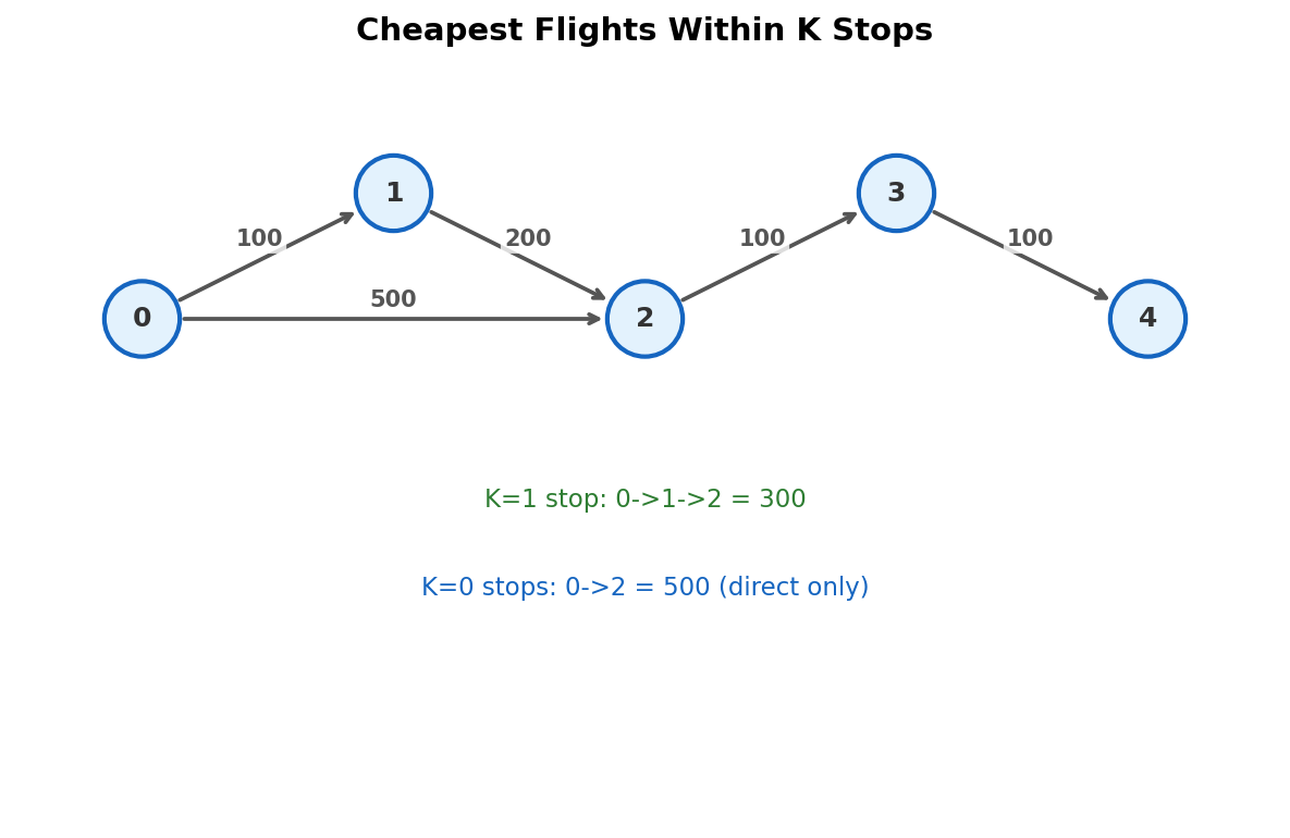
\(N\) cities, directed flights with prices. Find the cheapest price from src to dst using at most \(K\) intermediate stops (meaning at most \(K + 1\) edges).
Constraints: \(N \le 100\), flights \(\le N(N-1)/2\), \(K \le N - 1\).
The Bellman-Ford Connection
Bellman-Ford relaxes all edges in rounds. After round \(i\), you have the shortest paths using at most \(i\) edges. This is exactly what "at most K stops" asks for.
Run \(K + 1\) rounds of relaxation. After the last round, dist[dst] is the cheapest path using at most \(K + 1\) edges.
int findCheapestPrice(int n, vector<vector<int>>& flights,
                      int src, int dst, int k) {
    const int INF = 1e9;
    vector<int> dist(n, INF);
    dist[src] = 0;

    for (int i = 0; i <= k; i++) {
        vector<int> next(dist); // snapshot current distances
        for (auto& f : flights) {
            int u = f[0], v = f[1], w = f[2];
            if (dist[u] != INF) {
                next[v] = min(next[v], dist[u] + w);
            }
        }
        dist = next;
    }
    return dist[dst] == INF ? -1 : dist[dst];
}
Gotcha. You must copy
distintonextbefore each round. If you relax in-place, updates from the current round contaminate later relaxations, effectively allowing more edges than intended. This is the classic Bellman-Ford-with-rounds mistake.
Trace: Bellman-Ford with K = 1
Graph: 4 cities. Flights: 0->1 (100), 1->2 (100), 0->2 (500), 2->3 (100). Source: 0, destination: 3, \(K = 1\).
\(K + 1 = 2\) rounds (at most 2 edges).
| dist[0] | dist[1] | dist[2] | dist[3] | |
|---|---|---|---|---|
| Init | 0 | INF | INF | INF |
| Round 1 (1 edge) | 0 | 100 | 500 | INF |
| Round 2 (2 edges) | 0 | 100 | 200 | 600 |
After round 2: dist[3] = 600. Path: \(0 \to 2 \to 3\) (500 + 100), using 1 intermediate stop.
Note: the path \(0 \to 1 \to 2 \to 3\) costs 300 but uses 2 intermediate stops, exceeding \(K = 1\).
State-Expanded Dijkstra Approach
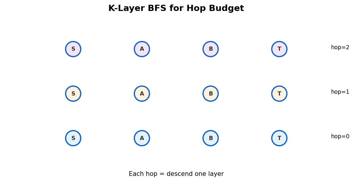
Alternatively, expand the state to (city, hops_used):
int findCheapestPrice(int n, vector<vector<int>>& flights,
                      int src, int dst, int k) {
    vector<vector<pair<int,int>>> adj(n);
    for (auto& f : flights)
        adj[f[0]].push_back({f[1], f[2]});

    vector<vector<int>> dist(n, vector<int>(k + 2, INT_MAX));
    priority_queue<tuple<int,int,int>,
                   vector<tuple<int,int,int>>,
                   greater<>> pq;
    dist[src][0] = 0;
    pq.push({0, src, 0});

    while (!pq.empty()) {
        auto [d, u, h] = pq.top(); pq.pop();
        if (u == dst) return d;
        if (d > dist[u][h]) continue;
        if (h > k) continue;
        for (auto [v, w] : adj[u]) {
            if (d + w < dist[v][h + 1]) {
                dist[v][h + 1] = d + w;
                pq.push({d + w, v, h + 1});
            }
        }
    }
    return -1;
}
Both approaches give the same answer. The tradeoffs:
| Approach | Complexity | Better when |
|---|---|---|
| Bellman-Ford | \(O(K \cdot E)\) | \(K\) is small, graph is dense |
| State-expanded Dijkstra | \(O(K \cdot V \cdot \log(K \cdot V))\) | Graph is sparse, many edges are heavy |
For LC 787 with \(N \le 100\), both are fast. For larger constraints, choose based on the density.
Obstacle Budget: LC 1293 Revisited
"You can eliminate at most K obstacles." This is a resource dimension with the same structure as hops.
State: (row, col, obstacles_remaining).
Transition: moving to cell \((r', c')\) costs 1 step. If the cell is an obstacle, it also costs 1 unit of budget. If budget drops below 0, the move is illegal.
int nrem = rem - grid[nr][nc]; // grid value is 0 or 1
if (nrem >= 0 && dist[nr][nc][nrem] == -1) {
    dist[nr][nc][nrem] = dist[r][c][rem] + 1;
    q.push({nr, nc, nrem});
}
Key insight. "At most K of something" is always a resource dimension. K stops, K obstacle removals, K teleports, K toll-free edges. The pattern is the same: add a dimension of size \(K + 1\) to your distance table.
The General Pattern
| Problem phrase | Resource | State |
|---|---|---|
| "at most K stops" | hops used | (node, hops) |
| "remove at most K obstacles" | removals left | (node, removals) |
| "at most K free edges" | freebies left | (node, freebies) |
| "arrive by time T" | time used | (node, time) |
| "use at most B budget" | budget left | (node, budget) |
Every row in this table is the same algorithm with a different resource name.
When K Is Large
If \(K\) approaches \(|V|\) or \(|E|\), the expanded state space becomes as large as the original problem without constraints. At that point, the budget is effectively unlimited, and you should just run plain Dijkstra/BFS.
For LC 1293 specifically: if \(K \ge R + C - 3\) (where \(R\) and \(C\) are grid dimensions), you can always walk a Manhattan-distance path and remove every obstacle along the way. The answer is just \(R + C - 2\).
This early exit prevents TLE on test cases with large \(K\) and small grids.
Gotcha. When \(K\) is very large relative to the graph size, state expansion wastes memory and time. Always check if the budget exceeds the maximum possible need.
LC 1928: Minimum Cost to Reach Destination in Time
\(N\) cities, roads with travel times and passing fees. Each city charges a fee to pass through. Reach city \(N-1\) from city \(0\) within time \(T\). Minimize the total fees paid.
State: (city, time_used). Resource: time budget.
This flips the usual setup: the "cost" you minimize (fees) is different from the resource you track (time). The Dijkstra priority queue sorts by fees, while the state tracks time.
// Transition: from (u, t) to (v, t + travel_time)
// if t + travel_time <= maxTime
// cost = fees[v]
if (t + tt <= maxTime && dist[u][t] + fees[v] < dist[v][t + tt]) {
    dist[v][t + tt] = dist[u][t] + fees[v];
    pq.push({dist[v][t + tt], v, t + tt});
}
Key insight. The resource dimension and the Dijkstra cost don't have to be the same thing. You can minimize fees while tracking time as a resource, or minimize time while tracking coins as a resource. The expansion is the same either way.
Trace: LC 787 with State-Expanded Dijkstra
Graph: 0->1 (100), 1->2 (100), 0->2 (500), 2->3 (100). \(K = 1\).
| Step | Pop (cost, city, hops) | Updates |
|---|---|---|
| 1 | (0, 0, 0) | dist[1][1]=100, dist[2][1]=500 |
| 2 | (100, 1, 1) | h=1, k=1, can still traverse. dist[2][2]=200 |
| 3 | (200, 2, 2) | h=2 > k=1, skip (exceeded stops) |
| 4 | (500, 2, 1) | dist[3][2]=600 |
| 5 | (600, 3, 2) | city==dst, return 600 |
Answer: 600. Same as Bellman-Ford.
Exercises
-
Bellman-Ford vs Dijkstra. On a graph with 1000 nodes, 5000 edges, and \(K = 3\), which approach is faster? What about \(K = 500\)?
-
Combining budgets. A problem says "at most K stops, and at most B budget." What is your state? What is the total state space?
-
No negative cycles. Why doesn't Bellman-Ford need a negative-cycle check for LC 787? (Hint: all flight prices are positive.)
-
Monotonicity. In the state-expanded Dijkstra for hops, is
dist[city][h] <= dist[city][h+1]always true? Construct a counterexample.
Problems
| Problem | Link | Difficulty |
|---|---|---|
| LC 787 — Cheapest Flights Within K Stops | leetcode.com/problems/cheapest-flights-within-k-stops | Medium |
| LC 1293 — Shortest Path in a Grid with Obstacles Elimination | leetcode.com/problems/shortest-path-in-a-grid-with-obstacles-elimination | Hard |
| LC 1928 — Min Cost to Reach Destination in Time | leetcode.com/problems/minimum-cost-to-reach-destination-in-time | Hard |
| AtCoder past202010_j | atcoder.jp/contests/past202010-open/tasks/past202010_j | Hard |