Time-Dependent Edges
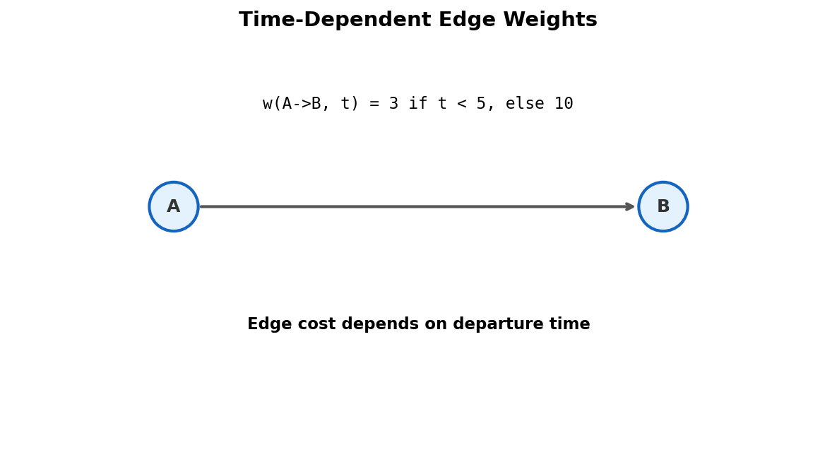
You're at the train station at 7:03 AM. The next train leaves at 7:10. You wait 7 minutes, ride for 20, arrive at 7:30. Your friend arrives at 7:10 sharp --- no wait, arrives at 7:30 too. Same edge, same train, same arrival. But if she'd arrived at 7:11, she'd wait until 7:20, arriving at 7:40. The edge cost changed because the clock changed.
Welcome to time-dependent graphs. The edge weight isn't a fixed number. It's a function of when you get there.
The Setup: AtCoder abc192_e (Train)
\(N\) cities, \(M\) bidirectional train lines. Train line \(i\) connects cities \(A_i\) and \(B_i\). Trains depart at times \(0, K_i, 2K_i, 3K_i, \ldots\) and take \(T_i\) time to travel. Find the earliest arrival time from city \(S\) to city \(T\).
The twist: you arrive at city \(u\) at time \(t\). The next train on line \(i\) departs at the smallest multiple of \(K_i\) that is \(\geq t\). You can't board a train that already left.
The Wait Calculation
This is the core mechanic. You arrive at time \(t\) and need the next departure at a multiple of \(K\).
In integer arithmetic, ceiling division of \(t\) by \(K\) is:
Then your arrival at the other end is:
Key insight. The edge cost from \(u\) to \(v\) is not \(T\) --- it's \(\text{next\_depart} - t + T\). The wait time depends on \(t\), so the same edge has different costs for different arrivals.
Why Dijkstra Still Works
Time-dependent edge costs could break Dijkstra. If traveling later made edges cheaper (cost decreases over time), then popping a node early wouldn't guarantee optimality. But here, the cost function satisfies a critical property:
If you arrive later, you depart no earlier. Formally, for any edge, if \(t_1 \leq t_2\), then \(\text{arrive}(t_1) \leq \text{arrive}(t_2)\).
Proof: if \(t_1 \leq t_2\), then \(\lceil t_1/K \rceil \leq \lceil t_2/K \rceil\), so the departure and arrival are both non-decreasing.
This is called the FIFO property (first-in, first-out). It guarantees Dijkstra's greedy choice remains correct.
Gotcha. Not all time-dependent problems have the FIFO property. Lesson 2 covers a case where waiting can be cheaper --- and Dijkstra still works, but for a subtler reason.
The State
Here's what's surprising: the state is just (city). No extra dimension. No layers.
Why? Because Dijkstra processes nodes in order of earliest arrival time. Once you pop city \(u\) with time \(t\), any later arrival at \(u\) would produce equal or worse departures on every outgoing edge. So dist[u] = t is final.
vector<long long> dist(n, LLONG_MAX);
dist[s] = 0;
priority_queue<pair<long long,int>,
               vector<pair<long long,int>>,
               greater<>> pq;
pq.push({0, s});

while (!pq.empty()) {
    auto [t, u] = pq.top(); pq.pop();
    if (t > dist[u]) continue;
    for (auto& [v, T, K] : adj[u]) {
        long long depart = ((t + K - 1) / K) * K;
        long long arrive = depart + T;
        if (arrive < dist[v]) {
            dist[v] = arrive;
            pq.push({arrive, v});
        }
    }
}
The values in the priority queue are arrival times, not abstract distances. But Dijkstra doesn't care --- it just sees non-negative numbers.
Trace: 4-City Example
Cities: 1, 2, 3, 4. Source = 1, Target = 4. Time starts at 0.
| Line | Cities | T (travel) | K (frequency) |
|---|---|---|---|
| A | 1 -- 2 | 3 | 5 |
| B | 1 -- 3 | 7 | 4 |
| C | 2 -- 4 | 2 | 3 |
| D | 3 -- 4 | 1 | 6 |
Initial: dist = [0, INF, INF, INF].
| Step | Pop (time, city) | Edge | Wait calc | Arrive | Update? |
|---|---|---|---|---|---|
| 1 | (0, 1) | A: 1->2 | depart = ceil(0/5)*5 = 0 | 0 + 3 = 3 | dist[2] = 3 |
| 1 | (0, 1) | B: 1->3 | depart = ceil(0/4)*4 = 0 | 0 + 7 = 7 | dist[3] = 7 |
| 2 | (3, 2) | C: 2->4 | depart = ceil(3/3)*3 = 3 | 3 + 2 = 5 | dist[4] = 5 |
| 3 | (5, 4) | target reached | --- | --- | --- |
| 4 | (7, 3) | D: 3->4 | depart = ceil(7/6)*6 = 12 | 12 + 1 = 13 | 13 > 5, skip |
Answer: 5.
Path: 1 -> 2 -> 4. Depart city 1 at time 0, arrive city 2 at time 3, catch the next train at time 3 (exact multiple of 3), arrive city 4 at time 5.
Notice city 3's route: arrive at time 7, but the next train departs at time 12 (next multiple of 6). That 5-minute wait kills this path.
The Ceiling Division Trick
This pattern appears constantly in competitive programming. Memorize it:
In C++:
For this problem, the next departure is ceil_div(t, K) * K. If \(t\) is already a multiple of \(K\), the train is right there --- no wait.
Gotcha. Watch out for \(t = 0\). When \(K = 5\),
ceil(0/5) * 5 = 0. The first train departs at time 0, which is correct. But if the problem says "trains depart at times \(K, 2K, 3K, \ldots\)" (starting from \(K\), not 0), then you needceil_div(t+1, K) * Kinstead. Read the problem statement carefully.
What dist[u] Actually Means
In standard Dijkstra, dist[u] is the shortest distance. Here, dist[u] is the earliest arrival time at city \(u\). The priority queue orders by arrival time. The relaxation check asks: "can I arrive at \(v\) earlier than the best known?"
This reframing is important. If the problem asks "what is the minimum travel time?", the answer is dist[T] - 0 (arrival minus departure). If it asks "what is the earliest arrival?", the answer is just dist[T].
Key insight. In time-dependent Dijkstra, the priority queue values are timestamps, not costs. The algorithm is the same --- only the interpretation changes.
When the Start Time Isn't Zero
Some problems say "you start at time \(t_0\)." Just initialize dist[s] = t_0 instead of 0. Everything else stays the same. The ceiling division handles the first wait correctly.
If the problem says "you can depart at any time \(\geq 0\) and want to minimize arrival time", the answer is still starting at time 0 --- because the FIFO property guarantees that leaving earlier never hurts.
Complexity
Same as standard Dijkstra: \(O((N + M) \log N)\). No state expansion needed. The only extra work per edge is one ceiling division --- \(O(1)\).
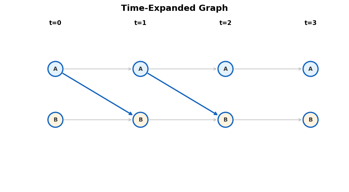
This is what makes time-dependent Dijkstra elegant. The graph isn't physically expanded. The time dependence is absorbed into the edge-weight computation.
Exercises
-
Wait time. You arrive at time \(t = 13\) and \(K = 5\). What is the next departure? What if \(t = 15\)?
-
FIFO check. An edge has travel time 10 but a discount: if you depart between times 5 and 8, the travel time drops to 2. Does this satisfy FIFO? Can you use Dijkstra directly?
-
Multiple lines. City \(u\) has two train lines to city \(v\): line A with \(T=3, K=7\) and line B with \(T=5, K=2\). You arrive at \(u\) at time 11. Which line gets you to \(v\) faster?
Problems
| Problem | Link | Difficulty |
|---|---|---|
| AtCoder abc192_e --- Train | atcoder.jp/contests/abc192/tasks/abc192_e | Medium |
| LC 1976 --- Number of Ways to Arrive at Destination | leetcode.com/problems/number-of-ways-to-arrive-at-destination | Medium |